Download
1 / 22
220 likes | 354 Vues
MMA708 – Analytical Finance II –Jan R. M. Röman. BLACK-DERMON-TOY MODEL WITH FORWARD INDUCTION. Wei Wang Maierdan Halifu Yankai Shao. INTRODUCTION. Black-Derman-Toy model (a short rate model) is a model of the evolution of the yield curve.

E N D
MMA708 – Analytical Finance II –Jan R. M. Röman BLACK-DERMON-TOY MODELWITH FORWARD INDUCTION Wei Wang Maierdan Halifu Yankai Shao
INTRODUCTION • Black-Derman-Toy model (a short rate model) is a model of the evolution of the yield curve. • It is a single stochastic factor (the short rate) determines the future evolution of all interest rates. • The parameters can be calibrated to fit the current term structure of interest rates (yield curve) and volatility structure as derived from implied prices (Black-76) for interest rate caps. • The model was introduced by Fischer Black, Emanuel Derman, and Bill Toy in the Financial Analysts Journal in 1990.
THEORETICAL BACKGROUND Key features of BDT-model • Its fundamental variable is the annualized one-period interest rate. The changes in short-rate derive all security prices. • Yield Curve - array of long rates (zero-coupon bonds yield) for various maturities. Volatilities Curve - array of yield volatilities for the same bonds. As input, both two curves come form the term structure. • The model varies an array of means and an array of volatility changes, the future volatility changes, the future mean reversion changes.
THEORETICAL BACKGROUND The short rate is given by the following process: the factor in front of ln(r) is the speed of mean reversion (gravity) θ(t) divided by the speed of mean reversion is a time-dependent mean-reversionlevel. • Advantage: Percentage as volatility unit for market convention. • Disadvantages: Due to log-normality, analytic solutions for bonds or bond options prices are not available. Numerical procedures are required to derive the short-rate tree that correctly returns the market term structures.
A STEP-TO-STEP SOLUTION • Example: Consider the value of an American call option on a five-year zero-coupon bond with time to expiration of four years and a strike price of 85.50. • How to price this option with following inputs?
A STEP-TO-STEP SOLUTION The price tree and its corresponding rate tree
A STEP-TO-STEP SOLUTION • Valuing Securities: assume that all expected returns are equal, lend money at r A One-Step Tree
A STEP-TO-STEP SOLUTION • Getting Today’s Prices from Future Prices We first derive prices 1 step in the future from prices 2 steps in the future with the same method above.
A STEP-TO-STEP SOLUTION • We find the prices of the zero-coupon bonds with maturity from one year to five year in the future. • Therefore we get the following table of data
A STEP-TO-STEP SOLUTION • Derive a 2-step tree by Risk-neutral valuation approach • In a standard binomial tree, we have
A STEP-TO-STEP SOLUTION • In the Black-Derman-Toy tree, the rates are assumed to be log-normally distributed. This implies • The solutions can be found by numeric method (Newton-Raphson method)
A STEP-TO-STEP SOLUTION • 2-step tree of prices and rates
A STEP-TO-STEP SOLUTION When we move further to a four-step tree, we must remember that the Black-Derman-Toy model is built on the following assumptions: • Rates are log-normally distributed. • The volatility is only dependent on time, not on the level of the short rates. There is thus only one level of volatility at the same time step in the rate tree.
A STEP-TO-STEP SOLUTION • Using the same method, we found the missing information in the two-period rate tree. The consecutive time steps can be computed by forward induction, introduced by Jamshidian (1991). 4-period rate tree as inputs to solve 5-period price tree
EXCEL/VBA APPLICATION • Data: We are aimed to create BDT-trees of a zero coupon bond with maturity 10.75years, time step (Delta) = 0.25, in this case, zero coupon yield and its volatility are given in the data. • Yield Curve: To examine the relationship between interest rate and time to maturity in each step, we therefore made a yield curve.
EXCEL/VBA APPLICATION • Rate Tree VBA: We developed following user-defined functions to calculate BDT matrix with VBA. • Function Bzero - calculates zero coupon bond yields based on continuously compounded interest rates. • Function BDTtree - determines the rate tree according to BDT model, which depends upon the parameters volatility, face value, delta as well as bond prices represented by the previous function Bzero on a continuous basis. Newton-Raphson method has been used during the calculation in order to optimize the algorithm. • Function Bond – calculates bond prices by the inputs face value, interest rate, periods, and delta ( time step).
EXCEL/VBA APPLICATION • Part of BDT Matrix
EXCEL/VBA APPLICATION Results: Rate Tree
EXCEL/VBA APPLICATION Results: Bond Tree
SUGGESTIONS FOR FURTHER READING • T.G., Bali, Karagozoglu, Implementation of the BDT-Model with Different Volatility Estimators, Journal of Fixed Income, March 1999, pp.24-34 • Fischer Black, Piotr Karasinsky, Bond and Option Pricing when Short Rates are lognormal, Financial Analysts Journal, July-August 1991, pp.52-59 • John Hull, Alan White, New Ways with the Yield Curve, Risk, October 1990a
Thank you for your attention