Download

1 / 14
140 likes | 301 Vues
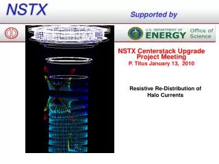
NSTX. Supported by. NSTX Centerstack Upgrade Project Meeting P. Titus Sept 1, 2010. Status of Disruption Simulations. nsel,s,loc,z,-100,-1.8 d,all,volt,0 ! Constrains the Volts DOF at the Lower CHI/Bellows/Ceramic Break. cpdele,all,all cpcyc,volt,.001,5,0,60,0. nodein1=10140

E N D
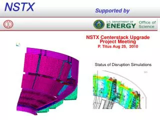
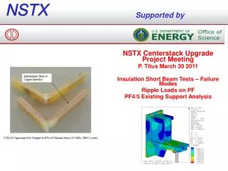
NSTX Supported by NSTX Centerstack Upgrade Project Meeting P. Titus Sept 1, 2010 Status of Disruption Simulations
nsel,s,loc,z,-100,-1.8 d,all,volt,0 ! Constrains the Volts DOF at the Lower CHI/Bellows/Ceramic Break cpdele,all,all cpcyc,volt,.001,5,0,60,0
nodein1=10140 nodein2=10553 nodein3=20932 nodein4=41709 *if,inum,gt,7,then HaloCur=700000./6/4 *endif *if,inum,gt,10,then HaloCur=.1/6/4 *endif f,Nodein1,amps,HaloCur f,Nodein2,amps,HaloCur f,Nodein3,amps,HaloCur f,Nodein4,amps,HaloCur Volt=0 !Output times [s]: t1=1.00E-03 $t2=5.00E-03$t3=5.50E-03$t4=6.00E-03$t5=6.50E-03$t6=7.00E-03$t7=7.50E-03$t8=8.00E-03$t9=8.50E-03$t10=9.00E-03 t11=9.50E-03$t12=1.00E-02$t13=1.10E-02$t14=1.20E-02$t15=1.30E-02$t16=1.40E-02$t17=1.50E-02$t18=1.60E-02$t19=1.70E-02$t20=1.80E-02$t21=1.90E-02 t22=2.00E-02$t23=2.10E-02$t24=2.20E-02$t25=2.30E-02$t26=2.40E-02$t27=2.50E-02$t28=2.60E-02$t29=2.70E-02$t30=2.80E-02$t31=2.90E-02$t32=3.00E-02 t33=3.50E-02$t34=4.00E-02$t35=4.50E-02$t36=5.00E-02$t37=5.50E-02$t38=6.00E-02$t39=6.50E-02$t40=7.00E-02$t41=7.50E-02$t42=8.00E-02$t43=8.50E-02 t44=9.00E-02$t45=9.50E-02$t46=1.00E-01$t47=1.50E-01$t48=2.00E-01
We have Eliminated the Poloidal Background Field from Ron’s Simulation Background Poloidal Fields Must Now be Added.
Set Background Fields From Hatcher/Woolley Zero Plasma Results from Plots Prepared by Joe Boales BackBz = -.4 !BackBz will be constant every only if BackBr=0. Otherwise it is constant just on z=z0 to satisfy Div(B)=0 BackBr = -.3 z0=-.6 ! height at which Br is truly radial for Bz & BtR = 0
time,.001 lswrite,1 *do,inum,1,44,1 time,t%inum%+100 *dim,vect%inum%,table,81,81,1,x,z,,5 ! Specfies a 81X 81 parameter table *tread,vect%inum%,'VecPot_case_%inum%','txt' ! Reads the file 1.txt into the table nall BR=130000*12*3*2e-7 ! Toroidal current *get,nmax,node,,num,max *do,i,1,nmax z=nz(i) x=nx(i) ! Applying Poloidal Fields !d,i,ay,vect%inum%(x,z) ! Intrepolates and applies the Vector Potential on the node !/x removed because Ron's Files have been corrected for 1/r d,i,ay,BackBz*x/2-BackBr*(z-z0)+vect%inum%(x,z) ! Intrepolates and applies the Vector Potential on the node !/x removed because Ron's Files have been corrected for 1/r !d,i,ay,BackBz*x/2-BackBr*(z-z0)! Applies only the background fields ! Applying the Toroidal Field d,i,az,-0.5*BR*log(x*x) ! applies vector potential for toroidal magnetic field *enddo d,all,ax,0. *if,inum,gt,7,then HaloCur=700000./6/4 *endif *if,inum,gt,10,then HaloCur=.1/6/4 *endif f,Nodein1,amps,HaloCur*.1 f,Nodein2,amps,HaloCur*.1 f,Nodein3,amps,HaloCur*.1 f,Nodein4,amps,HaloCur*.1 !f,nodeout,amps,-HaloCur*.1 lswrite,inum+1 *enddo Initial No Field Load Step Shift Time to Produce Low Bdot Read in Table Data Prepared by Ron (Mid-Plane Disruption Use Art Brooks Commands to Superimpose Appropriate A’s to Hatcher Disruption No More 1/r Correction Turn Halo Currents On and Off at Appropriate Times
Currents Flowing in the Passive Plates, Mid-Plane Disruption, Plasma 1 The upper bound of measured net currents [3] in the primary passive plates is also about 10% of the plasma current. Currents in the secondary passive plates are not as readily determined from the current vector plot but it is clear that they are lower, consistent with measured data. The OPERA axisymmetric Analysis produces only toroidal currents.The results of the Opera/ANSYS disruption simulation show eddy currents in the plates. In the ANSYS results there is a clear net toroidal current in the primary passive plates represented by larger current densities at the top of the plate than at the bottom. Based on the top and bottom current densities, at the time in the disruption that produced the largest current densities , the conduction cross section of the primary passive plates and an assumed triangular current density distribution: Fraction of IP flowing in the Primary Passive Plates is: (.467e9-.311e9)*5.4848e-3/4 /2E6 = .107 [3] "Characterization of the Plasma Current quench during Disruptions in the National Spherical Torus Experiment" S.P. Gerhardt, J.E. Menard and the NSTX Team Princeton Plasma Physics Laboratory, Plainsboro, NJ, USA Nucl. Fusion 49 (2009) 025005 (12pp) doi:10.1088/0029-5515/49/2/025005
Mid Plane Disruption =Plasma 1 Current Inventory in OPERA/ANSYS Disruption Analyses
$t5=6.50E-03 $t10=9.00E-03 ½ Period= 2.5 millisec, Frequency=1/.005=200
Mid Plane Disruption =Plasma 1 Static Structural Results No Halo Dynamic Results at the Edge of the PP. Peak Stress = 135MPa vs. 180 for Static Analysis
Mid Plane Disruption =Plasma 1 Dynamic Static: 2000 Mpa Dynamic: 700 MPa Static
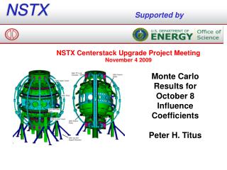
Mid Plane Disruption =Plasma 1 Lower Passive Plate Bolting Dynamic Results Results need to be adjusted for element size – but 130 Mpa peak and 70 Mpa Average looks Promising
Mid Plane Disruption =Plasma 1 Actual Vertical Field is ~.4T