Download
1 / 61
640 likes | 738 Vues
Primer on hydrologic models. Dennis P. Lettenmaier Department of Civil and Environmental Engineering University of Washington for presentation at Dividing the waters: Science for Judges Workshop IV Workshop on Climate Change Modeling: General Circulation Models and Hydrometeorologic Models

E N D
Primer on hydrologic models Dennis P. Lettenmaier Department of Civil and Environmental Engineering University of Washington for presentation at Dividing the waters: Science for Judges Workshop IV Workshop on Climate Change Modeling: General Circulation Models and Hydrometeorologic Models Hotel Boulderado Boulder, Colorado May 13 – 15, 2007
Some caveats All models are wrong, but some are useful G.E.P. Box, 1979 With poor assumptions, a man can make more mistakes in a millisecond than he could with common sense in a lifetime … unknown Beware those who believe their models D.P. Lettenmaier, 2007
Some background on runoff generation mechanisms • Saturation excess (also “Dunne Mechanism”) – runoff is generated only from areas for which the surface is hydraulically connected to the channel system, meaning saturated areas (which are dynamic at both seasonal and storm time scales). Most common locations: humid and semi-humid environments, especially forested. • Infiltration mechanism (also Horton overland flow) – occurs when rainfall intensity exceeds infiltration rate, causing (at least local) overland flow. Most common locations: urban areas; arid areas with e.g. crusted soils and high precipitation intensities; some agricultural areas (especially in summer).
Seasonal contraction of saturated area at Sleepers River, VT following snowmelt (source: Dunne and Leopold)
Expansion of saturated area during a storm (source: Dunne and Leopold)
Seasonal contraction of pre-storm saturated areas, Sleepers River VT (source: Dunne and Leopold)
The hydrologic modeling problem: Predict Q (streamflow) given P (precipitation), and perhaps other land surface meteorological variables (temperature, downward solar and longwave radiation, etc) Approaches: • “Black box” models: given sequence of Q and P, “train” a relationship • Examples: unit hydrograph (applicable to storm runoff prediction), regression (applicable to longer periods, e.g., seasonal or annual) • Shortcomings: • No physical causality • Most such models are linear, but nonlinearities govern hydrologic response under many conditions • Extrapolation beyond observed ranges of forcing and response data (extreme droughts, floods)
Example: Application of linear regression to seasonal runoff forecasting in the western U.S. (Apr-Aug runoff as a function of Apr 1 observed snow water content)
Classification of Hydrological Models Deterministic Stochastic Physically Based Conceptual Empirical Probabilistic Time series Distributed Lumped Grid based Subwatershed No distribution Source: USDA/ARS, Tucson, AZ
Modeling approaches (cont.) • Rainfall-runoff modeling (aka “conceptual hydrologic modeling”, “physically based modeling” • Essentially all models in this class are temporally distributed (typically meaning time steps hours to a day) • Subcategories: • Event (primarily storm) • Continuous (e.g., multi-years)* • Spatially lumped • Spatially distributed (or semi-distributed)*
Model characteristics • “Engineering” models – typically prescribe P and potential evapotranspiration (PET or Ep), which usually implies that vegetation is not represented explicitly. Engineering models generally are not concerned with causality, but rather in producing the most accurate predictions • Physically based models – typically represent vegetation explicitly, and often energy, as well as water cycle. Models that represent both water and energy fluxes often are designed for, or adapted from, land schemes in coupled land-atmosphere models (used for weather and climate prediction).
Some questions to ask: • What is the model’s conceptual basis (black box, physically based)? • If physically based, what mechanisms are represented (e.g., saturation vs infiltration excess runoff generation, or both)? • How is vegetation represented (explicitly, or in terms of PET)? • How was the model calibrated (calibration and verification periods, NSE, time series examples, mass balance, correlation with obs, etc)? • What is the basis for assuming applicability beyond the range of observations?
Some examples of physically based or conceptual hydrologic models: • HSPF/BASINS (EPA) – derivative of Stanford model of 1960s, the first time-continuous conceptual simulation model, generalized but still no explicit vegetation representation • NWSRFS (Sacramento) – another derivative of Stanford model; time continuous, used primarily for flood forecasting. No explicit representation of vegetation. • SWAT (USDA) – a quasi-conceptual time-continuous model built around SCS curve number variation of unit hydrograph method; vegetation/land cover links to PET and curve number represented • KINEROS (USDA) – a physically based, event model (physics mostly pertain to infiltration excess overland flow prediction; no representation of vegetation due to event nature) • Variable Infiltration Capacity (VIC) model – designed for coupled and uncoupled land-atmosphere and hydrologic prediction for large river basins. Represents both the water and energy cycles. Includes SVAT (soil-vegetation-atmosphere transfer scheme) representation of vegetation. It is spatially semi-distributed.
Hydrologic simulation modeling – the Stanford Watershed model (per Steve Gorelik and Keith Loague, Stanford University)
USDA Soil Water Assessment Tool (SWAT) Source: USDA/ARS, Tucson, AZ
(KINEROS) Kinematic Runoff & Erosion Model • Event-based (< minute time steps) • Distributed: physically-based model with dynamic routing • Hydrology, erosion, sediment transport • Smaller watersheds (< 100 km2) • Not applicable for snow • Primary Parameters • Area • Slope • Manning’s n • Percent Cover • Interception • Saturated Hydraulic Conductivity • Soil texture (% sand, silt, clay) • Pavement 71 72 73 74 Source: USDA/ARS, Tucson, AZ
¶ ¶ h Q + = - i f ¶ ¶ t x Excess Runoff From a Plane rainfall intensity (i) - KINEROS flow depth (h) Finite difference step length (dx) infiltration (f) q OtherFactors interception channel element hydraulic roughness rain splash erosion soil cohesion (erodibility) Source: USDA/ARS, Tucson, AZ Q
Automated Watershed Characterization the influence of CSA on watershed complexity area is removed due to presence of pond that never spilled during simulation period Note channel initiation Point changing with CSA 2.5% = 19.6 ha 1.5% = CSA of 11.8 ha N 0 1 km 5% = 39.3 ha 10% = 78.6 ha watershed 11, Walnut Gulch Experimental Watershed Source: USDA/ARS, Tucson, AZ
Macroscale modeling: A strategy for hydrologic modeling of large (e.g. continental) riverbasins ref. e.g. B. Nijssen et al, Streamflow Simulation for Continental-Scale Watersheds, Water Resources Research, 1997. Traditional “bottom up” hydrologic modeling approach (subbasin by subbasin)
Macroscale modeling approach (“top down”) 1 Northwest 5 Rio Grande 10 Upper Mississippi 2 California 6 Missouri 11 Lower Mississippi 3 Great Basin 7 Arkansas-Red 12 Ohio 4 Colorado 8 Gulf 13 East Coast 9 Great Lakes
Investigation of forest canopy effects on snow accumulation and melt Measurement of Canopy Processes via two 25 m2 weighing lysimeters (shown here) and additional lysimeters in an adjacent clear-cut. Direct measurement of snow interception
Calibration of an energy balance model of canopy effects on snow accumulation and melt to the weighing lysimeter data. (Model was tested against two additional years of data)
Summer 1994 - Mean Diurnal Cycle Rnet Rnet 300 Rnet 100 -100 250 H H 150 H 50 -50 120 LE LE LE 60 0 0 3 6 9 12 15 18 21 24 0 3 6 9 12 15 18 21 24 0 3 6 9 12 15 18 21 24 Observed Fluxes Simulated Fluxes Rnet Net Radiation H Sensible Heat Flux LE Latent Heat Flux Point Evaluation of a Surface Hydrology Model for BOREAS SSA Mature Black Spruce NSA Mature Black Spruce SSA Mature Jack Pine Flux (W/m2) Local time (hours)
Eurasia North America ) 20 10 2 km 6 16 8 12 6 snow cover extent (10 8 4 4 2 0 0 J F M A M J J A S O N D J J F M A M J J A S O N D J Month Month Observed Simulated Range in Snow Cover Extent Observed and Simulated
UPPER LAYER SOIL MOISTURE Illinois soil moisture comparison 0.40 TOPLATS regional ESTAR distributed X TOPLATS distributed 0.30 X SOIL MOISTURE (%) X X X X 0.20 X X X X X X X X X X 0.10 June 18th-July 20th, 1997 11:00 CST JUNE 20, 1997 11:00 CST JULY 12 1997 50 50 10 10 ESTAR TOPLATS ESTAR TOPLATS
A B C D 200 Soil Moisture (mm) Normalized 100 0 J F M A M J J A S O N D J J F M A M J J A S O N D J J F M A M J J A S O N D J J F M A M J J A S O N D J E F G H 200 Soil Moisture (mm) Normalized 100 0 J F M A M J J A S O N D J J F M A M J J A S O N D J J F M A M J J A S O N D J J F M A M J J A S O N D J Observed Simulated 60°N 60°N E H A D G 50°N 50°N B C F 40°N 40°N 20°E 30°E 40°E 50°E 60°E 70°E 80°E 90°E 100°E 110°E 120°E 130°E 140°E Mean Normalized Observed and Simulated Soil Moisture Central Eurasia, 1980-1985
Cold Season Parameterization -- Frozen Soils Key Observed Simulated 5-100 cm layer 0-5 cm layer
Macroscale hydrology models – implementation for large continental river basins
Model calibration (parameter estimation) • Applicable to conceptual/physically based models (parameter estimation for e.g. statistical models has stronger theoretical basis) • Most model parameters have some physical basis, typically used to place bounds on feasible range • Some model parameters are often constrained to literature values, in some cases based on sensitivity analysis that shows limited sensitivities • Other parameters subject to search – usually manual, sometimes via automated search procedures • Split sample approach of calibration vs verification periods is the norm, to avoid model overfitting • Simplifications are often made to reduce dimensionality of search problem, especially for distributed or semi-distributed models (where some parameters may be made identical spatially) • Objective function for search is usually (although doesn’t have to be) single valued, related to difference between predicted and observed runoff
Calibration criteria • Correlation obs – simulated (problem: linear multiples yield perfect correlation; lags can greatly reduce correlation) • Bias (necessary for water balance, but not sufficient) • Nash-Sutcliffe efficiency [1 – sum(sim – obs)2/variance(obs)] – most commonly used • Various multivariate measures
Infiltration: bi (more identifiable in dry climates) Baseflow: Ds Ws Dsmax Other: Soil Depths (particularly the baseflow layer) Ks expt (exponent n in Brooks –Corey eqn – describes variation of Ksat with soil moisture ‘global precip multiplier’ VIC model -- Typical Calibration Parameters Alternative Parameter Formulation • Nijssen parameters (select • model converts from D1, D2, D3 and D4 back to Ds, Ws, Dsmax and c • Ds = D1*D3 / D2 • Dsmax = D2*(1/(max moisture-D3))^D4 + D1*D3 • Ws = D3/(max layer moisture) • c = D4 (exponent in infiltration curve, usually set to 2) D1 linear reservoir coeff; D2 nonlinear res coeff; D3 threshold for switch See: Demaria et al., 2007, Monte Carlo Sensitivity Analysis of land surface parameters using the VIC model, JGR (in review)
www.hydro.washington.edu/Lettenmaier/Models/VIC/Documentation/Optimization.htmlwww.hydro.washington.edu/Lettenmaier/Models/VIC/Documentation/Optimization.html • “Mocom-UA” • very general structure for routine, although this makes code structure confusing Automatic Calibration (Optimization) shell script runs optimization calls C-program Mocom-UA Mocom-UA: - generates initial parameter samples calls shell script to: - run VIC - calculate statistics - [etc – anything else you want, e.g., plot] loop until done Mocom-UA: - evaluates stats from runs, generates new params calls shell script to run VIC … etc.