Download

1 / 40
410 likes | 544 Vues
The Sunspot Cycle: Long-Range Predictions for Long-Range Propagation. Dr. David H. Hathaway NASA MSFC Space Science Office 2014 January 11 GARS TechFest 2014. Outline. The Sun and Solar Activity The Sun and the Ionosphere The Sunspot Cycle The Sun’s Magnetic Dynamo

E N D
The Sunspot Cycle:Long-Range Predictions forLong-Range Propagation Dr. David H. Hathaway NASA MSFC Space Science Office 2014 January 11 GARS TechFest 2014
Outline • The Sun and Solar Activity • The Sun and the Ionosphere • The Sunspot Cycle • The Sun’s Magnetic Dynamo • Sunspot Cycle Predictions
The Sun Radius = 109 REarth Mass = 333,000 MEarth Surface Temp = 9,930 °F Surface Density = Air/5000 Core Temp = 28 million °F Core Density = Gold × 8 Composition: 70% H 28 % He 2% (C, N, O…)
Sunspots Sunspots are dark (and cooler) regions on the surface of the Sun. They have a darker inner region (the Umbra) surrounded by a lighter ring (the Penumbra). Sunspots usually appear in groups that form over hours or days and last for days or weeks. The earliest sunspot observations indicated that the Sun rotates once in about 27 days.
Sunspot Structure Sunspots are regions where intense magnetic fields break through the surface of the Sun. The magnetic field strengths are typically about 6000 times stronger than the Earth’s magnetic field.
Explosive Events • Solar flares – 10-1000X excess in X-rays and Extreme Ultraviolet (EUV) • Coronal Mass Ejections (CMEs) – magnetic clouds blasted off the Sun • Solar Energetic Particles – relativistic particles from flares and CMEs
CME Impact on Earth Magnetized clouds of plasma blasted off of the Sun as CMEs can impact the Earth’s environment – distorting the magnetic field surrounding the Earth and producing energetic particles that stream into the Earth’s atmosphere to create aurorae.
Space Weather Space weather refers to conditions on the Sun and in the space environment that can influence the performance and reliability of space-borne and ground-based technological systems, and can endanger human life or health.
The Basics Extreme Ultraviolet (EUV) and X-rays from the Sun ionize the gases in the Earth’s upper atmosphere. At night the ions and electrons recombine at the denser lower altitudes (the D and E layer) where collisions are more frequent. The D layer disappears at night. The E layer (or patches of the E layer) can survive the night if the solar EUV is strong. Solar EUV varies with the sunspot cycle – strong at max.
The Solar Spectrum Solar ultraviolet light (UV) is energetic enough to dissociate O2 molecules and form O3 (ozone) in the stratosphere. It takes Extreme Ultraviolet (EUV and XUV) to ionize atoms and molecules in the ionosphere. N2 -> N2+ + e- for λ < 80 nm O -> O+ + e- for λ < 91 nm O2 -> O2+ + e- for λ < 103 nm NO -> NO+ + e- for λ < 134 nm EUV produces the F-region XUV (+ Ly β) produces the E-region X-rays (+ Ly α) produce the D-Region Ly β = 102.6 nm, Ly α = 121.6 nm He 30.4 Ly α The solar spectrum from X-rays to Microwaves
Solar Cycle EUV Variability Measurements of the flux of radio waves at 10.7 cm (2.8 GHz) have been made three times daily since 1947 from sites in Canada. This is often used as a proxy for solar EUV to characterize the ionospheric forcing. However, measurements of the actual EUV emissions indicate some deviations – in particular at the last cycle minimum. 30.4 nm
TIMED SEE The Solar EUV Experiment (SEE) on the NASA Thermosphere Ionosphere Mesosphere Energetics and Dynamics (TIMED) mission was designed to fill in this “EUV Hole”. TIMED was launched in 2002 and is still operating. Wavelength coverage (2004) XUV Variability 2002-2013
MUF and TEC The Maximum Usable Frequency (MUF) for radio waves reflected off of the ionosphere is directly related to the Total Electron Content (TEC) of the ionosphere. The TEC depends upon both the solar EUV and X-ray irradiance and geomagnetic activity. We now have direct observations of solar EUV/XUV/X-ray emissions – no need for proxies!
Sunspot Cycle Discovery Astronomers had been observing sunspots for over 230 years before Heinrich Schwabe, an amateur astronomer in Dessau, Germany, discovered in 1844 that the number of sunspot groups and the number of days without sunspots increased and decreased in cycles of about 10-years. Schwabe’s data for 1826 to 1843 Number of Sunspot Groups per Year Number of Spotless Days
23 Full Cycles Shortly after Schawbe discovery Rudolf Wolf proposed using a “Relative” Sunspot Number count. While there were many days without observations prior to 1849, sunspots have been counted on every day since. To this day we continue to use Wolf’s Relative Sunspot Number and his cycle numbering. The average cycle lasts about 11 years, but with a range from 9 to 14. The average amplitude is about 100, but with a range from 50 to 200.
Sunspot Latitudes Sunspots appear in two bands on either side of the equator. These bands drift toward the equator as the cycle progresses. Big cycles have wider bands that extend to higher latitudes. Cycles typically overlap by 2-3 years.
Sunspot Group Tilt- Joy’s Law Sunspot groups are tilted with the leading spots (the spots seen first as the Sun rotates) closer to the equator than the following spots. In 1919 Alfred Joy noted that this tilt increases with latitude on the Sun.
Hale’s Magnetic Polarity Law In 1919 George Ellery Hale found that the magnetic field in sunspots followed a definite law, “Hale’s Law” such that: “…the preceding and following spots … are of opposite polarity, and that the corresponding spots of such groups in the Northern and Southern hemispheres are also opposite in sign. Furthermore, the spots of the present cycle are opposite in polarity to those of the last cycle”.
Three Solar Cycles in Action In addition to these magnetic polarity changes and the equatorward drift of the sunspot latitudes, there are important flows on the surface and within the Sun: Differential Rotation– faster at the equator, slower near the poles; and Meridional Flow – flow from the equator toward the poles along the surface.
Polar Field Reversals In 1958 Horace Babcock and Bill Livingston noted that the magnetic polarities of the Sun’s weak polar fields also reverse from one cycle to the next, and that this reversal happens at about the time of sunspot cycle maximum (the South reversed in 1957 the North in 1958).
Babcock’s Dynamo (1961) Dynamo models have been developed to explain the sunspot cycle. a) Dipolar field at cycle minimum threads through a shallow layer below the surface. b) Differential rotation shears out this poloidal field to produce a strong toroidal field (first at the mid-latitudes then progressively lower latitudes). c) Buoyant fields erupt through the photosphere giving Hale’s polarity law and Joy’s Law. d) Meridional transport cancels preceding polarities across the equator and carries following polarity to the poles.
Polar Fields – Seeds for Cycles The Sun’s polar fields are the seeds of the next solar cycle in these dynamo models. We have direct observations for the last three cycles and a proxy (polar faculae) for the last 10 cycles.
Polar Fields as Predictors There is a strong correlation between polar fields and the amplitude of the next solar cycle (hemisphere by hemisphere in terms of peak sunspot area). North – Blue squares South – Red circles Cycles 21-23 are from direct magnetic measurements. Earlier cycles are from counting polar faculae.
Polar Field Prediction forCycle 24 Small Cycle 24 predicted by Polar Fields (Svalgaard, Cliver, & Kamide, 2005)
Four Years Ago - Minimum Small Cycle 24 predicted.
This Year - Maximum This is the Maximum of Cycle 24! The polar fields built up during Cycle 23 were a good predictor.
How are Polar Fields Made? Back to Babcock (1961) a) Dipolar field at cycle minimum threads through a shallow layer below the surface. b) Differential rotation shears out this poloidal field to produce a strong toroidal field (first at the mid-latitudes then progressively lower latitudes). c) Buoyant fields erupt through the photosphere giving Hale’s polarity law and Joy’s Law. d) Meridional transport cancels preceding polarities across the equator and carries following polarity to the poles.
Polar Field Production Variations in sources: more sunspots – more polar field Variations in source details: more tilt – more polar field Variations in poleward flow: faster flow – more polar field Option 1 is the most important – cycles will get bigger (or smaller) in series until something (Option 2 or 3) breaks the trend.
Polar Field Production I Cycles with more sunspots should produce stronger polar fields which leads to another strong cycle … some other variation is needed to modulate/regulate this process. Otherwise the cycles would either grow without limit or decay to nothing. We do see long term trends in cycle size – they tend to get bigger and then smaller over 100-year intervals. Something stops their growth and something starts them growing again.
Polar Field Production II Dasi-Espuig et al. (2010) found that the average tilt, <α>, of sunspot groups changed with cycle amplitude. The small tilt seen in big Cycle 19 may have stopped the further growth of the sunspot cycles to produce a much smaller cycle 20. 15 16 17 18 19 20 21 Solid line - <α> from Mt. Wilson Observatory Dash-Dot line - <α> from Kodaikanal Observatory Dashed line – sunspot area from Greenwich Observatory
Polar Field Production III We have made measurements of the Meridional Flow of magnetic elements since 1996 and find significant variations. The Meridional flow is fast at cycle minima and slow at cycle maxima. The slow-down at cycle maxima depends on cycle strength – much slower in Cycle 23 than in Cycle 24. The faster flow in Cycle 24 should help to make stronger polar fields and a bigger Cycle 25. 21 22 23
The Prognosis for Cycle 25 Cycle 24 has far fewer (and smaller) sunspots than Cycles 22 and 23. Although the faster Meridional flow should help overcome this deficit, the slow rate of change in the polar fields strongly suggests that polar fields that will build up over the rest of Cycle 24 will still be very weak.
Conclusions • Solar activity impacts modern technology • Solar EUV/XUV emissions and magnetic disturbances control the ionosphere • We are making progress in understanding the Solar Cycle • Cycle 24 is at its peak – the smallest in 100 years. • Cycle 25 may be even smaller yet!