Download
1 / 28
280 likes | 388 Vues
CORC. Integrated boundary current observations in the global climate system. Investigators: U.Send, R.Davis, D.Rudnick, B.Cornuelle, D.Roemmich, P. Niiler. NOAA OCO System Review, Silver Spring, 29 October 2010. OceanObs09: “boundary currents are a critical gap”. CORC objective:

E N D
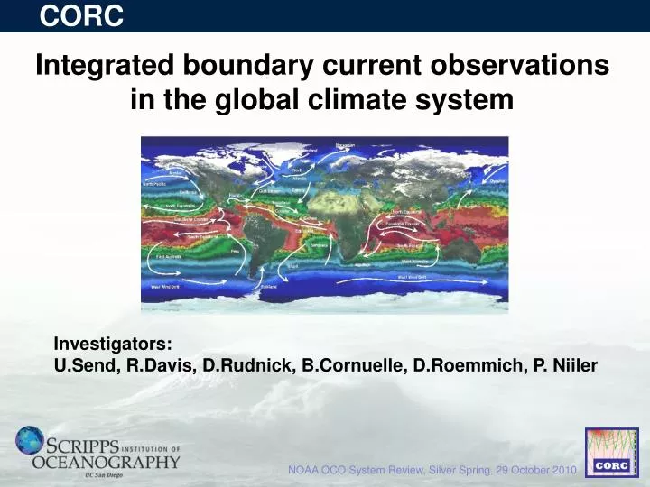
CORC Integrated boundary current observations in the global climate system Investigators: U.Send, R.Davis, D.Rudnick, B.Cornuelle, D.Roemmich, P. Niiler NOAA OCO System Review, Silver Spring, 29 October 2010
OceanObs09: “boundary currents are a critical gap” • CORC objective: • develop and demonstrate efficient integrated technologies and methodologies to fully characterize and observe • western boundary currents- major factor in driving climate - societal relevance by understanding and forecasting • eastern boundary currents- major impact of climate - societal relevance by understanding and for management/mitigation • After an intensive phase in a region, leave behind a reduced efficient system.
Technology developments in CORC Bottom-release “pop-up” surface drifters (7 released sequentially from 2000m depth this year). Acoustic data retrieval from long-term lower-cost fixed subsurface instrumentation
Acoustic data recovery success with gliders • typical data transfer: 10-15kb/dive • up to 7km distance • 3-month mission transferred 2.7Mb, 1.8Mb good data One of the 5 sites has problems, probably sidewall reflections
Western Boundary Current in the Solomon Sea (feeding EUC) typical glider path see Kessler poster bottom pressure • now 2 gliders in water at any time • large transport variability, similar to ARGO • relation to La Nina/El Nino • remove eddy noise and add higher temporal sampling by adding modem PIES across basin in the future
Testbed and Eastern Boundary Current site: California Current 66 glider mooring XBT glider 90 surface drifters mooring • - Integrate glider, XBT, mooring, drifter obs. • - Staggered coverage from coast to interior • - Capitalize from CalCOFI data, merge with altimeter and ARGO • - state estimate from adjoint model
XBT and ARGO sampling, connecting to basin interior PX37 off San Francisco (20 yr record)- northward undercurrent +2.5Sv mean- southward Calif Current -5.5Sv mean- banded structure is persistent PX37S off closer to line 90, 2 years data now- similar transports- more structure and larger flow than CalCOFI
Glider alongshore flow: mean and 0-500m variability Line 80 Line 90 3 years of glider data now Line 90
El Nino signal in glider observations of the California Current Equatorial SST Anomalies averagedover 200km along line 90(T, isopycnal depth, S, v) wind and curl
Mooring transports, flow profile, reference level, bottom pressure Geostrophic transport very sensitive toreference level bottom pressure gradientscontribute 1Sv to transport mean flow profile,zero near 300m. Deeper ref level givessouthward bias
Water column heat content from moorings and IES Co-located mooring and IES IES only Co-located mooring and IES
CORC surface drifter observations and analyses Mean surface flow from drifters 1992-2008 1 year of CORC drifter trajectories
CORC state estimates via MITgcm adjoint assimilation • MITgcm model description: • 6km resolution, 72 levels, 20min timestep • 4DVar adjoint • initial&boundary cond from MIT ECCO • atmosphere from NCEP NAM • data from Jan’07 - Jul’09:- altimetry and satellite SST - ARGO& ship hydrography (CalCOFI) - glider T&S, XBT - mooring T&S - soon IES, bottom pressure, drifters • control variables:- IC’s and BC’s - surface forcing • dynamically consistent state estimates • ongoing improvements/iterations (#90 now) Model domain (gray box)
Model-mooring and model-glider comparison for mean flow glider mooring model model
Model-mooring and model-glider comparison for time-dependent flow glider model mooring model
Wind stress curl field diagnosed from state estimate Needed model to estimate wind stress curl… inshore curl isopycnal depth(2 month lag)
CORC model state estimate improves shortwave heatflux The model managed to correct shortwave heat flux using in-situ observations NCEP NAM Rms difference between new Cayan&Iacobellis satellite product and various estimates Cayan product NAM adjusted by adjoint
CORC model state estimate products page (used by NOAA SWFSC) Cannot rely on single proxy or measurement for managing fisheries (e.g. Temp in Southern California Bight, relation can break down). See Ned Cyr presentation.
New short-term (17day) assimilation experiments using ROMS • Model • 9km horizontal resolution nested in 18km • Initial and boundary conditions from OCCA • Surface forcing fields were from NCEP NAM • assimilation 2008.10.11 to 2080.10.28 • corrects initial condition, wind forcing, surface heat flux and the open boundary • Observations • Alongtrack sea surface height data (AVISO) • Sea surface temperature (AVHRR) • CalCOFI temperature and salinity • Mooring data • glider data • ARGO Short runs allow “operational” data assimilation
Snapshots of alongshore flow field in short-term assimilation
Normalized cost for glider/mooring data after 9 iterations glider T mooring T glider S mooring S Section transport timeseries
Conclusions and proposed next phase • large variability in flow and transport, dominated by eddies and Rossby waves • by summer 2011 will have 5½ years of glider data and 3 years of mooring/PIES can analyze low-frequency transports and compare with XBT/ARGO • adjoint model/state estimates will be brought to consistency with data • short-term “now-cast” technique will be refined • research ongoing into constraining transports more directly • Next phase: • develop capability for capturing the upwelling overturning circulation • add alongshore resolution for constraining 4-D field • study trade-off and efficiencies between XBT, gliders, moorings, bottom pressure sensors • deliver weekly estimates of upwelling circulation • seasonal hindcasts of physical system driving ecosystem and OA • maps onto Lindstrom requirements/societal drivers and outputs
Roemmich ’89, Bograd et al ’01 upwelling overturning transports
Integrated glider and mooring sampling plan CORC present glider occupations of box Daily glider sections moorings for daily nettransport estimates SCCOOS Close transport inshoreof 500m isobath “Peter” add existing lines foralongshore resolution CORC present resolve alongshorestructure/connectivity (“Peter Niiler memorial”) Geostrophic moorings, possibly virtual moorings
Space-time sampling of gliders and CalCOFI in the California Current Line 90