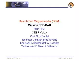
THEMIS SCIENCE WORKING TEAM MEETING Search Coil Magnetometer (SCM) team

1. THEMIS SCIENCE • WORKING TEAM MEETING • Search Coil Magnetometer (SCM) team • Co-i: A. Roux, O. Le Contel • Technical Manager(*): C. Coillot • Lead Engineer: A. Bouabdellah • Technicians: D. Alison & S. Ruocco • Software Engineers: P. Robert & (X) • (*) SCM team thanks Bertrand de la Porte who was the first • technical manager and for his continuing support. • CETP-Vélizy, France

2. SCM objectives • SCM will measure the magnetic components of waves associated with substorm breakup. Wave signature is essential to identify the mechanism responsible for triggering breakup. • Wave signatures are also expected to play a critical role in plasma transport through the magnetotail and across the magnetopause.

3. SCM overview (I) • The SCM 3-axis antennas are located at the end of 1 meter SCM boom • Magnetic components: 3 analogs signals from 0.1 Hz to 4kHz. • Sensitivity: 0.8pT/Hz@10Hz; 0.02pT/  Hz@1kHz • Weight: 570 g • Pre-amplifier (in 3D technology), located inside s/c body. • Weight: 200 g • Power: 75 mW • PA + sensors: • First qualified at CETP (vibrations, thermal cycling) and then at UCB/JPL on s/c. • Fully calibrated at CETP quiet facility near Chambon la Forêt.

4. SCM overview (II) • Calibration mode • A Triangular signal generated by the PA and applied to a feedback winding installed in each antenna. • Once per orbit a calibration is run for 30 seconds (default). • After 60 seconds, the calibration is automatically turned off.

5. SCM calibration processing (I) Waves calibration method 1) get Level 1SCM waveform (in Volts) 2) Select a time interval for calibration (Selecting this time interval is required to apply FFT and calibrate ) Single Calibration In sensor coordinates 3) Production of "clean" raw waveforms in the spinning Sensor Coordinate System (SCS) (substract sinusoidal wawe at spin frequency via a ‘desinus’ software ; requires the knowledge of the spin frequency) 4 ) Calibration of each component and conversion in nT in the frequency domain (for the selected time interval) (FFT, Correction of tranfer function by *1/G(fi) ; cut-off at low frequency ) 5) Get calibrated time series data in nT, in the spinning Sensor Coordinate System (SCS) (FFT -1) 6) Waveform transformation from SCS to Despun System Change to Despun or other classical coordinate systems (Require Spin phase) 7) Waveform transformation from SCS to GSE System, or others (GSM, MAG, GEO…) (Require Rocotlib software or other)

6. SCM calibration processing (II) Making use of calibration method (Steps 1-5)

7. SCM science data (I) • Physical quantities (L2 data): • In DSC (Despun System Coord.), GSM and GSE coordinates • FS waveforms (scf) of Bx, By, Bz [8 S/s; All.~ 10.8h depending on which probe] • PB waveforms (scp) [128 S/s; All.~ 1.2h] • WB waveforms (scw) [8192 S/s; All.~ 43s] • Filterbank data (fbk) [1comp.; 6 freq.] throughout orbit • PB spectra (ffp) [2 comp.; 32 freq.] • WB spectra (ffw) [2 comp.; 64 freq.]

8. SCM science data (II) • L2 subset: • Magnetic field aligned frame (MFA) • Mininum variance frame (MVA) • Polarisation analysis Using FFT and assuming .B =0 and k   we can get the k direction and large and small ellipse axis directions z B0 k k  k 

9. SCM comments • Commissioning: • SCM should be turned on at the beginning in order to measure the noise generated by each instrument • SCM should be turned on with an operation mode allowing a good characterization of generated noise for instance with waveform at 256 S/s or may be short period at max. sample rate (16384 S/s)