Download
1 / 9
90 likes | 195 Vues
A better way of modeling ionospheric electrodynamics. Paul Withers Boston University (withers@bu.edu) Center for Space Physics Journal Club Tuesday (Monday) 2008.02.19

E N D
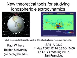
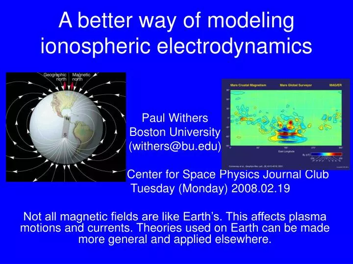
A better way of modeling ionospheric electrodynamics Paul Withers Boston University (withers@bu.edu) Center for Space Physics Journal Club Tuesday (Monday) 2008.02.19 Not all magnetic fields are like Earth’s. This affects plasma motions and currents. Theories used on Earth can be made more general and applied elsewhere.
How do textbooks calculate ion velocities in an ionospheric model ? • Two separate sections – vertical motion and horizontal motion • Vertical motion – weak magnetic field • No current. Vertical ambipolar diffusion. Non-zero Eparallel set by gravity and pressure gradients. • Vertical motion – strong magnetic field • No current. Ambipolar diffusion along fieldline. Non-zero Eparallel set by gravity and pressure gradients. • Horizontal motion – neglect gravity and pressure gradients • Currents are non-zero. Conductivity tensor relates currents and electric field. • Typical 3D model – mix assumptions • Use “horizontal” assumptions to show that Eparallel is zero, go to fieldline-integrated equations, solve for electric field. Re-introduce gravity and pressure gradients, find 3D ion motion • Why two sections?Why no intermediate magnetic field?Why mix assumptions?Why no general theory?
“Justification” of Assumptions – Relative Sizes of Terms • Nj (number density of charged species) from the continuity equation • Rate of change of Nj= Production - Loss • vj (species velocity) is given by the steady-state momentum equation • Gravity Pressure gradient Lorentz force Ion-neutral collisions Loss timescale vs. Transport timescale Gyrofrequency (qB/m) vs. What does this mean for the Collision frequency (vjn) terrestrial ionosphere?
Earth is not the only possible case • Mars z • Earth Strong field Weak field Transport Photochem Strong field Weak field Transport Photochem Ne Weak/strong transition occurs when vertical motion is irrelevant, so horizontal assumption seems reasonable Vertical plasma motion is important in weak field region, strong field region, and nasty transition (dynamo) region. Preceding assumptions fail badly.
Alternative Approach Y contains grav, pressure, E, etc Replace the nasty cross product Leads to equation for vj = …. Eventually get J/E relationship, generalization of Use div J = 0, curl of E = 0, plus boundary conditions to get equations that can be solved for E. Substitute solution for E in other equations to get J, vj, etc. Use vj in continuity equation to step Nj forward in time.
What are Q and S in ? • S is the usual conductivity tensor • Q is sum of gravity and pressure gradient terms • Direction of Q is vertical for weak field • Direction of Q is field-aligned for strong field Ratio of gyrofrequency to collision frequency defines Gravity and Pressure gradient Direction depends on Kj
vz using (solid line), vz using weak-field limit of ambipolar diffusion (dashed line), and vz using strong-field limit of ambipolar diffusion (dotted line). Application to a 1-D Mars-like model Very simple, Don’t over-interpret vz is negative below 150 km and positive above 150 km. vz transitions smoothly from the weak-field limit at low altitudes to the strong-field limit at high altitudes.
-Jx (dashed line), Jy (dotted line) and |J| (solid line). Jz = 0. Ke = 1 at 140 km, Ki = 1 at 200 km |J| is >10% of its maximum value between 150 km and 260 km Currents are significant within and above the 140 km – 200 km “dynamo region”
Conclusions • Conditions on Mars are outside parameter range common to terrestrial work • This forces re-examination of basic assumptions • can be generalized to • This formalism can handle 3D plasma motion and currents in any magnetic field strength