Download
1 / 12
120 likes | 308 Vues
One-way migration. Migration. There are two populations (x and y), each with a different frequency of A alleles (px and py). Assume migrants are from population x, and residents are population x; unidirectional).

E N D
Migration • There are two populations (x and y), each with a different frequency of A alleles (px and py). • Assume migrants are from population x, and residents are population x; unidirectional). • After migration, m is the migrant portion of the population y, and (1-m) is the resident portion of the population y. py’ is the p after migration: • py’ = m x px + (1-m) x py • dpy = m x px + (1-m) x py – py • dpy = m x px + py – m x py – py • dpy = m x px + m x py • dpy = m(px-py)
Change in allele frequency with one-way migration (m = 0.01)
Natural Selection • The interaction between alleles and environment shapes the direction of the change in allele frequencies resulting in evolution of adaptable traits.
Fitness and coefficient of selection (s) • Darwinian fitness is defined as the relative reproductive ability of a genotype. • The genotype that produces the most offspring is assigned a fitness (W) value of 1. Selection coefficient (s) equals (1-W) • AA produces on average 8 offspring • Aa produces on average 4 offspring • aa produces on average 2 offspring. • WAA = 1.0; sAA = 1-1 = 0 • WAa = 0.5; sAa = 1-0.5 = 0.5 • Waa = 0.25; saa = 1-0.25 = 0.75
How to calculate change in allele frequency after selection Wmean = p2 WAA + 2pq WAa + q2 Waa
Possibilities WAA = WAa = Waa: no natural selection WAA = WAa < 1.0 and Waa = 1.0: natural selection and complete dominance operate against a dominant allele. WAA = WAa = 1.0 and Waa < 1.0: natural selection and complete dominance operate against a recessive allele. WAA < WAa < 1.0 and Waa = 1.0: heterozygote shows intermediate fitness; natural selection operates without effects of complete dominance. WAA and Waa < 1.0 and WAa = 1.0: heterozygote has the highest fitness; natural selection/codominance favor the heterozygote (also called overdominance). WAa < WAA and Waa = 1.0: heterozygote has lowest fitness; natural selection favors either homozygote.
Selection against a recessive lethal phenotype • Recessive trait result in reduced fitness. • Frequency of the recessive allele decreases over time. • Not completely eliminated since present in heterozygotes.
Heterozygote superiority • Distribution of malaria and frequency of Hb-s allele leading to sickle cell disease in homozygotes.
Balance between mutation and selection • When an allele becomes rare, changes in frequency due to natural selection are small. • Mutation occurs at the same time and produces new rare alleles. • For a complete recessive allele at equilibrium: • q = √µ/s • If homozygote recessive is lethal (s = 1) then q = √µ
Model 1 • Simulate the change in allele frequencies directly by mathematical modeling of the forces that act on them. • Set initial values for p and q; • Set initial sample size (effective population size); • Set the HWE as the null model (p2 + 2pq + q2 = 1); • Allow for forces such as mutation rate, migration, genetic drift, and selection to act on the null model. • Estimate the change in allele frequencies over time using iterations (i.e., the program loops over for a number of generations as given by the arguments).
Model 2 • Simulate individuals of a population(s) having DNA sequence polymorphisms, and allow them to evolve randomly or under certain forces. • Set initial number of individuals (N at t = 0, equals to the effective size of the population, Ne); • Generate a null matrix for N x K x G, where K = 2 (diploid), and G equals to the number of genes considered (start with a single gene, if else assume genes are not linked for simplicity). • Set the total number of alleles (Nk, start with Nk = 2) for each G. • Set the initial number of homozygotes, heterozygotes for G. • Allow for the individuals mate randomly to produce offspring, iterate to simulate generations; for simplicity assume that all individuals die after reproduction. E.g., annual plants where Nt+1 = bNt + 0 Nt • Allow for forces to act on the null model, and test their effects on the allelic evolution.