Download
1 / 14
140 likes | 254 Vues
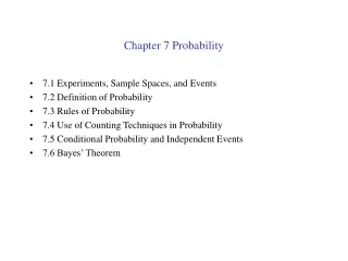
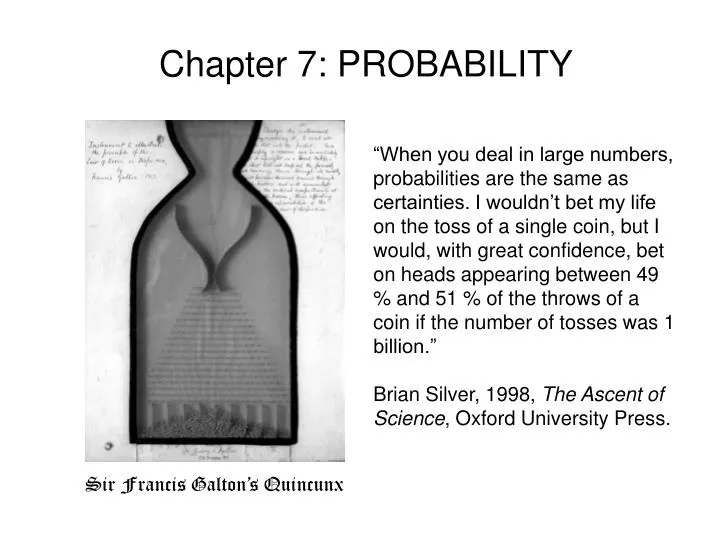
Chapter 7: PROBABILITY. “When you deal in large numbers, probabilities are the same as certainties. I wouldn’t bet my life on the toss of a single coin, but I would, with great confidence, bet on heads appearing between 49 % and 51 % of the throws of a coin if the number of tosses was 1 billion.”

E N D
Chapter 7: PROBABILITY “When you deal in large numbers, probabilities are the same as certainties. I wouldn’t bet my life on the toss of a single coin, but I would, with great confidence, bet on heads appearing between 49 % and 51 % of the throws of a coin if the number of tosses was 1 billion.” Brian Silver, 1998, The Ascent of Science, Oxford University Press. Sir Francis Galton’s Quincunx
Histogram Time record Histogram 10 digital values: 1.5, 1.0, 2.5, 4.0, 3.5, 2.0, 2.5, 3.0, 2.5 and 0.5 V resorted in order: 0.5, 1.0, 1.5, 2.0, 2.5, 2.5, 3.0, 3.5, 4.0 V N = 9 occurrences; j = 8 cells; nj = occurrences in j-th cell The histogram is a plot of nj (ordinate) versus magnitude (abscissa).
Proper Choice of Δx The choice of Δx is critical to the interpretation of the histogram. ← made using 3histos.m
Δx Choices Typically, we construct equal-width-interval histograms.
Histogram Construction Rules • To construct equal-width histograms: • Identify the minimum and maximum values of x and its range where xrange = xmax – xmin. • Determine K class intervals (usually use K = 1.15N1/3). • Calculate Δx = xrange / K. • Determine nj (j = 1 to K) in each Δx interval. Note ∑nj = N. • Check that nj > 5 and Δx ≥ ux. • Plot nj versus xmj,where xmj is the midpoint value of each interval.
Frequency Distribution The frequency distribution is a plot of nj /N versus magnitude. It is very similar to the histogram. ← made using hf.m Figure 7.7
Probability Density Function Concept • Consider a signal that varies in time. Figure 7.8 • What is the probability that the signal at a future time will reside between • x and x + Dx?
For x(t): fj /Dx • For n occurrences: Probability Density Function (pdf) • Definition:
In-Class Example • Determine the probability that x is between 1 and 7.
A consequence of this is that PDF pdf Figure 7.14 Probability Distribution Function (PDF) • The probability distribution function (PDF) is related to the integral of the pdf.
When the pdf is ‘normalized’ correctly: Normalization of the pdf Here, >> not normalized So, define pnew(x) = 1/3 p(x) such that
Integrating the pdf expressions give In-Class Example • Determine the expressions for the PDF curve, knowing that of the pdf curve.
The Normal pdf and PDF Figure 8.4