Download
1 / 66
670 likes | 843 Vues
ANOVA and Regression. Brian Healy, PhD. Objectives. ANOVA Multiple comparisons Introduction to regression Relationship to correlation/t-test. Comments from reviews. Please fill them out because I read them More examples and not just MS

E N D
ANOVA and Regression Brian Healy, PhD
Objectives • ANOVA • Multiple comparisons • Introduction to regression • Relationship to correlation/t-test
Comments from reviews • Please fill them out because I read them • More examples and not just MS • More depth on technical details/statistical theory/equations • First time ever!! • I have made slides from more in depth courses available on-line so that you have access to formulas for t-test, ANOVA, etc. • Talks too fast for non-native speakers
Review • Types of data • p-value • Steps for hypothesis test • How do we set up a null hypothesis? • Choosing the right test • Continuous outcome variable/dichotomous explanatory variable: Two sample t-test
Steps for hypothesis testing • State null hypothesis • State type of data for explanatory and outcome variable • Determine appropriate statistical test • State summary statistics • Calculate p-value (stat package) • Decide whether to reject or not reject the null hypothesis • NEVER accept null • Write conclusion
Example • In previous class, two groups were compared on a continuous outcome • What if we have more than two groups? • Ex. A recent study compared the intensity of structures on MRI in normal controls, benign MS patients and secondary progressive MS patients • Question: Is there any difference among these groups?
Two approaches • Compare each group to each other group using a t-test • Problem with multiple comparisons • Complete global comparison to see if there is any difference • Analysis of variance (ANOVA) • Good first step even if eventually complete pairwise comparisons
Global test-ANOVA • As a first step, we can compare across all groups at once • The null hypothesis for ANOVA is that the means in all of the groups are equal • ANOVA compares the within group variance and the between group variance • If the patients within a group are very alike and the groups are very different, the groups are likely different
Hypothesis test • H0: meannormal=meanBMS=meanSPMS • Outcome variable: continuous Explanatory variable: categorical • Test: ANOVA • meannormal=0.41; meanBMS= 0.34; meanSPMS=0.30 • Results: p=0.011 • Reject null hypothesis • Conclusion: At least one of the groups is significantly different than the others
Technical aside • Our F-statistic is the ratio of the between group variance and the within group variance • This ratio of variances has a known distribution (F-distribution) • If our calculated F-statistic is high, the between group variance is higher than the within group variance, meaning the differences between the groups are not likely due to chance • Therefore, the probability of the observed result or something more extreme will be low (low p-value)
This is the distribution under the null This small shaded region is the part of the distribution that is equal to or more extreme than the observed value. The p-value!!!
Now what • The question often becomes which groups are different • Possible comparisons • All pairs • All groups to a specific control • Pre-specified comparisons • If we do many tests, we should account for multiple comparisons
Type I error • Type I error is when you reject the null hypothesis even though it is true (a=P(reject H0|H0 is true)) • We accept making this error 5% of the time • If we run a large experiment with 100 tests and the null hypothesis was true in each case, how many times would we expect to reject the null?
Multiple comparisons • For this problem, three comparisons • NC vs. BMS; NC vs. SPMS; BMS vs. SPMS • If we complete each test at the 0.05 level, what is the chance that we make a type I error? • P(reject at least 1 | H0 is true) = a • P(reject at least 1 | H0 is true) = 1- P(fail to reject all three| H0 is true) = 1-0.953 = 0.143 • Inflated type I error rate • Can correct p-value for each test to maintain experiment type I error
Bonferroni correction • The Bonferroni correction multiples all p-values by the number of comparisons completed • In our experiment, there were 3 comparisons, so we multiply by 3 • Any p-value that remains less than 0.05 is significant • The Bonferroni correction is conservative (it is more difficult to obtain a significant result than it should be), but it is an extremely easy way to account for multiple comparisons. • Can be very harsh correction with many tests
Other corrections • All pairwise comparisons • Tukey’s test • All groups to a control • Dunnett’s test • MANY others • False discovery rate
Example • For our three-group comparison, we compare each and get the following results from Tukey’s test
Questions to ask yourself • What is the null hypothesis? • We would like to test the null hypothesis at the 0.05 level • If well defined prior to the experiment, the correction for multiple comparison if necessary will be clear • Hypothesis generating vs. hypothesis testing
Conclusions • If you are doing a multiple group comparison, always specify before the experiment which comparisons are of interest if possible • If the null hypothesis is that all the groups are the same, test global null using ANOVA • Complete appropriate additional comparisons with corrections if necessary • No single right answer for every situation
Correlation • Is there a linear relationship between IL-10 expression and IL-6 expression? • The best graphical display for this data is a scatter plot
Correlation • Definition: the degree to which two continuous variables are linearly related • Positive correlation- As one variable goes up, the other goes up (positive slope) • Negative correlation- As one variable goes up, the other goes down (negative slope) • Correlation (r) ranges from -1 (perfect negative correlation) to 1 (perfect positive correlation) • A correlation of 0 means that there is no linear relationship between the two variables
Hypothesis test • H0: correlation between IL-10 expression and IL-6 expression=0 • Outcome variable: IL-6 expression- continuous Explanatory variable: IL-10 expression- continuous • Test: correlation • Summary statistic: correlation=0.51 • Results: p=0.011 • Reject null hypothesis • Conclusion: A statistically significant correlation was observed between the two variables
Technical aside-correlation • The formal definition of the correlation is given by: • Note that this is dimensionless quantity • This equation shows that if the covariance between the two variables is the same as the variance in the two variables, we have perfect correlation because all of the variability in x and y is explained by how the two variables change together
How can we estimate the correlation? • The most common estimator of the correlation is the Pearson’s correlation coefficient, given by: • This is a estimate that requires both x and y are normally distributed. Since we use the mean in the calculation, the estimate is sensitive to outliers.
Distribution of the test statistic • The standard error of the sample correlation coefficient is given by • The resulting distribution of the test statistic is a t-distribution with n-2 degrees of freedom where n is the number of patients (not the number of measurements)
Regression-Everything in one place • All analyses we have done to this point can be completed using regression!!!
Quick math review • As you remember, the equation of a line is y=mx+b • For every one unit increase in x, there is an m unit increase in y • b is the value of y when x is equal to zero
Picture • Does there seem to be a linear relationship in the data? • Is the data perfectly linear? • Could we fit a line to this data?
How do we find the best line? • Linear regression tries to find the best line (curve) to fit the data Let’s look at three candidate lines • Which do you think is the best? • What is a way to determine the best line to use?
What is linear regression? • The method of finding the best line (curve) is least squares, which minimizes the distance from the line for each of points • The equation of the line is y=1.5x + 4
Example • For our investigation of the relationship between IL-10 and IL-6, we can set up a regression equation • b0 is the expression of IL-6 when IL-10=0 (intercept) • b1 is the change in IL-6 for every 1 unit increase in IL-10 (slope) • ei is the residual from the line
The final regression equation is • The coefficients mean • the estimate of the mean expression of IL-6 for a patient with IL-10 expression=0 (b0) • an increase of one unit in IL-10 expression leads to an estimated increase of 0.63 in the mean expression of IL-6 (b1)
Tough question • In our correlation hypothesis test, we wanted to know if there was an association between the two measures • If there was no relationship between IL-10 and IL-6 in our system, what would happen to our regression equation? • No effect means that the change in IL-6 is not related to the change in IL-10 • b1=0 • Is b1 significantly different than zero?
Hypothesis test • H0: no relationship between IL-6 expression and IL-10 expression, b1 =0 • Outcome variable: IL-6- continuous Explanatory variable: IL-10- continuous • Test: linear regression • Summary statistic: b1 = 0.63 • Results: p=0.011 • Reject null hypothesis • Conclusion: A significant correlation was observed between the two variables
Wait a second!! • Let’s check something • p-value from correlation analysis = 0.011 • p-value from regression analysis = 0.011 • They are the same!! • Regression leads to same conclusion as correlation analysis • Other similarities as well from models
Technical aside-Estimates of regression coefficients • Once we have solved the least squares equation, we obtain estimates for the b’s, which we refer to as • To test if this estimate is significantly different than 0, we use the following equation:
Assumptions of linear regression • Linearity • Linear relationship between outcome and predictors • E(Y|X=x)=b0 + b1x1 + b2x22is still a linear regression equation because each of the b’s is to the first power • Normality of the residuals • The residuals, ei, are normally distributed, N(0, s2) • Homoscedasticity of the residuals • The residuals, ei, have the same variance • Independence • All of the data points are independent • Correlated data points can be taken into account using multivariate and longitudinal data methods
Linear regression with dichotomous predictor • Linear regression can also be used for dichotomous predictors, like sex • Last class we compared relapsing MS patients to progressive MS patients • To do this, we use an indicator variable, which equals 1 for relapsing and 0 for progressive. The resulting regression equation for expression is
Interpretation of model • The meaning of the coefficients in this case are • b0 is the estimate of the mean expression when R=0, in the progressive group • b0 + b1is the estimate of the mean expression when R=1, in the relapsing group • b1 is the estimate of the mean increase in expression between the two groups • The difference between the two groups is b1 • If there was no difference between the groups, what would b1 equal?
Mean in wildtype=b0 Difference between groups=b1 Mean in Progressive group=b0
Hypothesis test • Null hypothesis: meanprogressive=meanrelapsing (b1=0) • Explanatory: group membership- dichotomous Outcome: cytokine production-continuous • Test: Linear regression • b1=6.87 • p-value=0.199 • Fail to reject null hypothesis • Conclusion: The difference between the groups is not statistically significant