Download
1 / 31
310 likes | 422 Vues
George Pouliot* and Thomas Pierce* Atmospheric Sciences Modeling Division/ARL/NOAA Tom Pace Office of Air Quality Planning and Standards/EPA 5 th Annual CMAS Conference October 17, 2006 *In partnership with the USEPA, National Exposure Research Laboratory.

E N D
George Pouliot* and Thomas Pierce* Atmospheric Sciences Modeling Division/ARL/NOAA Tom Pace Office of Air Quality Planning and Standards/EPA 5th Annual CMAS Conference October 17, 2006 *In partnership with the USEPA, National Exposure Research Laboratory Developing Emission Inventories for Biomass Burning for Real-time and Retrospective Modeling
Wildland Fire EmissionsSelected Acknowledgements • NOAA/ARL-RTP (R. Mathur) • NOAA/ARL-SS (R. Draxler) • NOAA/NESDIS (S. Kondragunta, X. Zhang, M. Ruminski) • NOAA/NWS (P. Davidson, J. McQueen) • NOAA/Research (S. Fine) • UNC-CEP (U. Shankar, J. Vukovich)
Biomass Burning Emissions • GOAL (1): Develop a method to estimate “real-time” biomass burning emissions for the EPA/NOAA Air Quality forecast system (PM2.5 and Ozone) • Key Issues • Fire locations • Fire size, fuel loading, and emission factors • “Forecasts” of biomass burning • Agricultural burning
Real-time Biomass Burning Emissions Questions • What accuracy in space and time is needed? • Is “persistence” sufficient? (We currently assume that current fires continue to burn for the next 48 h.) • Do we need a fire behavior model? • Can we use a simple “one-size-fits-all” model? • Can we combine different data sets and approaches to make a better forecast?
Real-time Biomass Burning Emissions • Existing data sources and methods: • BlueSky (U.S. Forest Service) • HySplit smoke plume estimates (NOAA/ARL) • Limited chemistry and physics • HMS simple approach (NOAA/EPA-AMD) • “One-size-fits-all” • Modified WF-Abba approach (NOAA-NESDIS) • Satellite-derived fire detects and fuel loading • Preliminary results for the last two will be discussed
“One Size Fits All” approach • Adapt “older” HySplit assumption that all fire detects use the same emission factor • Use SMOKE updates from the BlueSky-EM tool to create emissions for ETA/CMAQ system • Use daily/near-real-time Hazard Mapping System (HMS) product from NOAA/NESDIS for fire detects • Use the “raw” version of HMS product and not the HySplit version
“One Size Fits All” approach • Other Criteria Pollutants • Used 1996-2002 emission inventory for wildland fires • Created average ratios of other criteria pollutants to PM2.5 • “Derived” emission factors for other pollutants
“One Size Fits All” approach Wildland Fire Emission Factors (kg/ha)
“One Size Fits All” approach • Burn area for each “fire” set to 22.3 ha (based on analysis of EPA 2001 NEI dataset w/ total annual burn area and total number of fires). For operational forecasts, assume 16.7 ha/day (75% of total burn area). • Heat output (used for plume rise) set to 725 x 106 BTUs/day (based on an aggregated set of BlueSky simulations). • Diurnal profile for emissions from the WRAP. • PM2.5 emission factor set to 225 kg/ha (review of existing emission factors, which exhibit a wide range [20-800 kg/ha]). • 7 year average NEI factor range: 187-279 kg/ha
“One Size Fits All” approach ETA/CMAQ Test CaseJune 18-July 5, 2005 • 5x ETA/CMAQ system with PM version of CMAQ • “Cold” start used for some species, as only the PM-3x version of system avbl for June 2005 • 12 km grid/national domain • Major wildland fires in southwestern U.S. • Cave Creek Complex Fire: Second worst wildfire in the state of Arizona • Fire started in June 21, 2005 by a lightning strike • 243,950 acres burned
Cave Creek Complex Fire News Video of Fire on 22 June 2005 North of Carefree, AZ Source: http://www.abc15.com/gallery
Satellite View of Cave Creek Fire The Moderate Resolution Imaging Spectroradiometer (MODIS) on NASA's Terra satellite captured this image of the fire on June 23, 2005, at 11:50 a.m., local time Source: http://www.nasa.gov/vision/earth/lookingatearth/Arizona_Wildifire06.23.05.html
Fire Locations June 18-July 5, 2005: HMS and 209 Ground Reports Legend: Red=HMS and Ground Report Match Green= Ground Report Only Blue=HMS only Cave Creek Fire
Difference in Max 8-hr Ozone for June 25 Forecast HMS Fires Case – No Fire Case
Difference in 24-hr Average PM2.5 June 24 Forecast HMS Fires Case – No Fire Case
Scatter Plots of Max 1-hr Ozone, Max 8-hr Ozone and daily Mean PM2.5 for entire episode Note: only model-obs. pairs selected where we detected a fire impact: O3 (Fire-base)>4ppb PM25 (Fire-base)> 2ug/m3
Summary of”one size fits all” approach • Daily HMS product appears to reasonably capture large fires. • A preliminary system using HMS fire detects has been tested successfully. A final report has been delivered by UNC-CEP. • The fire emissions algorithm resulted in higher ozone and PM2.5 concentrations for a major fire event, which appear to agree more closely with observations than the base model. • Additional tests and comparisons with NESDIS (post-WF-ABBA-approach) are underway. • The preliminary system is ready for experimental real-time tests. • Other work could include improved characterization of fire size, fuel loading, emission factors, and temporal profiles.
NOAA/NESDIS Satellite derived Emission estimates • Developed by X. Zhang, S. Kondragunta, F. Kogan, J Tarpley, and W. Guo • NOAA/NESDIS has developed a new algorithm to derive biomass burning emissions of PM2.5 from remotely-sensed fire products in near-real-time for regional and global air quality modeling applications
NOAA/NESDIS Satellite- derived Emission estimates • Fuel loading • Fraction of fuel consumed • Emission factor • Fire locations • Fire size
Fuel Loading Database • Uses maximum monthly MODIS Leaf Area Index (LAI) and allometric models that relate leaf foliage biomass with other biomass components in forests, shrubs, and grasses Emission Factors • Determined from a fuel moisture category using AVHRR Normalized Vegetation Index (NDVI) product
NOAA/NESDIS Satellite derived Emission estimates • Work in progress • Still refining method to estimate fire size from satellite • Initial work so far is to look at fire locations and compare with ground reports • Plan to test ETA/CMAQ for same 2005 episode
Fire Locations June 18-July 9, 2005: NESDIS and 209 Ground Reports Legend: Red=NESDIS and Ground Report Match Green=NESDIS only Blue=Ground only
Fire Locations June 18-July 9, 2005: NESDIS and 209 Ground Reports Legend: Red=NESDIS and Ground Report Match Green=NESDIS only Blue=Ground only Cave Creek Fire
Biomass Burning Emissions Retrospective Modeling • GOAL (2): Develop a method to estimate biomass burning emissions for the National Emissions Inventory for years > 2002 (e.g. 2005) • The 2002 NEI for biomass burning is the most comprehensive to date • Many $$$ spent by RPOs to create this inventory • Develop a method for biomass emission inventory that is better than pre-2002 methods and not as costly as 2002
Biomass Burning Emissions Retrospective Modeling • What sources of data do we have for retrospective modeling? • 209 Reports • GOES satellite products • MODIS satellite products
Biomass Burning Emissions Retrospective Modeling Questions • How much detail do we need in the inventory? • Do we try to characterize only the largest fires accurately? • What satellite data should we use? • MODIS and/or GOES
Biomass Burning Emissions Retrospective Modeling Questions • How accurate are MODIS, GOES and 209 reports? • See A. Soja et. al. "How well do satellite data quantify fire and enhance biomass burning emissions estimates?"
Biomass Burning Emissions Retrospective Modeling Proposed Approach • Combine MODIS fire detects and 209 reports to get fire locations • Use land cover data to distinguish between ag burning, wildfires and Rx burning • Get fuel loading from a national database (FCCS or NFDRS) • Develop inventory for 2005 • Test methodology by redoing inventory for 2002 and compare to 2002 NEI
Biomass Burning Emissions • For forecasting air quality, we recommend a combination of available methods and data … but, fire behavior modeling will be needed for “true” forecasts • For retrospective air quality modeling, satellite-derived data offer much promise for capturing the temporal and spatial variation of large fires
Biomass Burning Emissions Disclaimer: The research presented here was performed under the Memorandum of Understanding between the U.S. Environmental Protection Agency (EPA) and the U.S. Department of Commerce’s National Oceanic and Atmospheric Administration (NOAA) and under agreement number DW13921548. Although it has been reviewed by EPA and NOAA and approved for publication, it does not necessarily reflect their views or policies.