Download
1 / 13
130 likes | 282 Vues
Scilab. Revisão – parte1. Vetores e Matrizes. Vetor Linha u = 0:3 = [0 1 2 3 ] Vetor Coluna u = [0; 1; 2; 3]. Funções. function [varRetorno1, ... , varRetornoN] = nomeDaFuncao(param1, ... , paramN) // corpo da função end function. Definindo função degrau. function[v] = degrau(t)

E N D
Scilab Revisão – parte1
Vetores e Matrizes Vetor Linha u = 0:3 = [0 1 2 3 ] Vetor Coluna u = [0; 1; 2; 3]
Funções function [varRetorno1, ... , varRetornoN] = nomeDaFuncao(param1, ... , paramN) // corpo da função end function
Definindo função degrau... function[v] = degrau(t) v = []; b = size(t); for u = [1:b(2)] if (t(u)>=0) then v = [v 1]; else v = [v 0]; end end endfunction Obs.: Nome de variável e função: SEM ACENTOS!
Operações com Sinais • Time Reversal φ(t) = pe(-t) • Time Shifting φ(t) = pe(t - 1) • Time Scaling φ(t) = pe(2.5*t) Função Plot: plot(t,degrau(t),color(“red”))
PolinÔmios • poly([roots], ‘v’) | poly([coef], ‘v’, ‘c’) p = poly([1 2], ‘s’) p = 2 - 3s + s2 q = poly([1 2], ‘s’, ‘c’) p = 1 + 2s • roots(q)
Análise de sistema contínuos (D2 + 3D + 2) y(t) = D x(t) D = poly(0,'D') P = D Q = D^2 + 3*D + 2 sysPol = syslin(‘c’, P, Q)
syslin(‘dom’,num,den) sysPol = syslin(‘c’, P, Q) linspace(start, end, numberOfSteps) t=linspace(0,10,500)
Simulação da convolução Covolução com Impulso: impresp = csim(‘imp’, t, sysPol) Covolução com Entrada qualquer: res = csim(<função entrada>, t, sysPol)
Exercicio 1: Defina o sinal x(t) abaixo e aplique as seguintes operações. Obs.: use cores diferentes para melhor visualização das transformações. a)x(t-4) b)x(2t) c)-x(-t)
Exercicio 02: Defina a função h(t) especificada pela equação abaixo e simule a covolução dela com a função definida no exercicio 1. (D2+6D+9)y(t) = (2D+9)x(t)
Terminando • Comando help; • Referências http://www.scilab.fr/doc/intro/intro.pdf http://www.scilab.fr/doc/signal.pdf http://www.scilab.fr/doc/lmidoc/lmi.pdf http://scilab.org/
Dúvidas huv@cin.ufpe.br