Download
1 / 19
230 likes | 603 Vues
Queueing Theory. What is a queue? Examples of queues: Grocery store checkout Fast food (McDonalds – vs- Wendy’s) Hospital Emergency rooms Machines waiting for repair Communications network. Queueing Theory. Basic components of a queue:. customers.

E N D
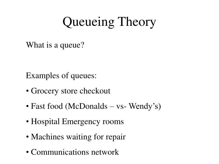
Queueing Theory • What is a queue? • Examples of queues: • Grocery store checkout • Fast food (McDonalds – vs- Wendy’s) • Hospital Emergency rooms • Machines waiting for repair • Communications network
Queueing Theory Basic components of a queue: customers Input source Queue Service (calling population) mechanism
Queueing Theory • Input source: • population size (assumed infinite) • customer generation pattern (assumed Poisson w rate or equivalently, exponential with an inter-arrival time ) • arrival behavior (balking, blocking) • Queue: • queue size (finite or infinite) • queue discipline (assumed FIFO, other include random, LIFO, priority, etc..)
Queueing Theory • Service mechanism: • number of servers • service time and distribution (exponential is most common)
Queueing Theory Naming convention: a / b / c a – distribution of inter-arrival times b – distribution of service time c – number of servers Where M – exponential distribution (Markovian) D – degenerate distribution (constant times) Ek – Erlang distribution (with shape k) G = general distribuiton Ex. M/M/1 or M/G/1
Queueing Theory Terminology and Notation: State of system – number of customers in the queueing system, N(t) Queue length – number of customer waiting in the queue - state of system minus number being served Pn(t) – probability exactly n customers in system at time t. s – number of servers ln – mean arrival rate (expected arrivals per unit time) when n customers already in system mn – mean service rate for overall system (expected number of customers completing service per unit time) when n customers are in the system. r – utilization factor (= l/sm , in general)
Queueing Theory Terminology and Notation: L = expected number of customers in queueing system = Lq = expected queue length = W = expected waiting time in system (includes service time) Wq = expected waiting time in queue
Queueing Theory Little’s Law: W = L / l and Wq = Lq / l Note: if ln are not equal, then l = l W = Wq + 1/m when m is constant.
Role of Exponential Distribution Let T be a random variable representing the inter-arrival time between events. fT(t) a Property 1: fT(t) is a strictly decreasing function of t (t> 0). P[0 <T<] > P[t<T<t +] P[0 <T< 1/2a] = .393 P[1/2a<T< 3/2a] = .383 Property 2: lack of memory. P[T > t + | T > ] = P[T > t] t fT(t) = ae-atfor t> = 0 FT = 1 - e-at E(T) = 1/a V (T) = 1/a2
Role of Exponential Distribution Property 3: the minimum of several independent exponential random variables has an exponential distribution. Let T1, T2,…. Tn be distributed exponential with parameters a1, a2,…, an and let U = min{T1, T2,…. Tn } then: U is exponential with rate parameter a = Property 4: Relationship to Poisson distribution. Let the time between events be distributed exponentially with Parameter a. Then the number of times, X(t), this event occurs over some time t has a Poisson distribution with rate at: P[X(t) = n] = (at)ne-at/n!
Role of Exponential Distribution Property 5: For all positive values of t, P[T<t + | T > t] for small . a can be thought of as the mean rate of occurrence. Property 6: Unaffected by aggregation or dis-aggregation. Suppose a system has multiple input streams (arrivals of customers) with rate l1, l2,…ln, then the system as a whole has An input stream with a rate l =
Birth-Death Process Birth – arrival of a customer to the system Death – departure of a customer from the system N(t) – random variable associated with the state of the system at time t (i.e. the number of customers, n, in the system at time t). Assumptions – customers inter-arrival times are exponential at a rate of ln and their service times are exponential at a rate of mn Queuing System Departures - mn Arrivals - ln
Rate Diagram for Birth-Death Process 0 1 2 n-2 n-1 n … …
Development of Balance Equations for Birth-Death Process M/M/1 System 0 1 2 n-2 n-1 n … …
Development of Balance Equations for Birth-Death Process M/M/s System – multiple servers 0 1 2 n-2 n-1 n … …
Development of Balance Equations for Birth-Death Process M/M/1/k System – finite system capacity 0 1 2 k-2 k-1 k …
Development of Balance Equations for Birth-Death Process M/M/1 System – finite calling system population 0 1 2 N-2 N-1 N …
M/G/1 Queue A system with a Poisson input, but some general distribution for service time. Only two characteristics of the service time need be known: the mean (1/m) and the variance (1/s2). P0 = 1 – r, where r = l/m Lq = L = r + Lq Wq = Lq/ lW = Wq + 1/ m