Download

1 / 61
620 likes | 811 Vues
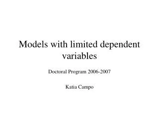
Models with limited dependent variables. Doctoral Program 2006-2007 Katia Campo. 3. Nested Logit Model. (K.Train, Ch.4, Franses and Paap Ch.5). 3. Nested Logit Model. Choice between J>2 alternatives which can be grouped into subsets based on differences in substitution pattern Example:.

E N D
Models with limited dependent variables Doctoral Program 2006-2007 Katia Campo
3. Nested Logit Model (K.Train, Ch.4, Franses and Paap Ch.5)
3. Nested Logit Model • Choice between J>2 alternatives which can be grouped into subsets based on differences in substitution pattern • Example: Choice of transportation mode Car Transit Carpool Bus Train Car alone
3. Nested Logit Model • Assumption cumulative distribution of error terms • Probability
3. Nested Logit Model • Probability can be decomposed into 2 logit models (1) (2)
3. Nested Logit Model • Link between Pni | Bk * Pn Bk (upper and lower model level) through inclusive value Ink • To comply with RUM k must be in the [0,1] interval • IIA within, not across nests
3. Nested Logit Model Estimation • Joint estimation • Sequential estimation • Estimate lower model • Compute inclusive value • Estimate upper model with inclusive value as explanatory variable Disadvantages sequential estimation • Add fourth step, using the parameter estimates as starting values for joint estimation
3. Nested Logit Model • Example: Location choices by French firms in Eastern and Western Europe • Dependent var.: probability of choosing location j Pj=P(πj> πk k≠j ) • Location choices are likely to have a nested structure (non-IIA) • First, select region (East or Western Europe) • Next, select country within region Disdier and Mayer (2004)
3. Nested Logit Model • Example 1: Location choices by French firms in Eastern and Western Europe Location choice E.Eur W.Eur ……… ……… CN C1 CJ+1 CJ Disdier and Mayer (2004)
3. Nested Logit Model • Location choices: Data • 1843 location decisions in Europe from 1980 to 1999 (official statistics) • 19 host countries (13 W.Eur, 6 E.Eur) Disdier and Mayer (2004)
3. Nested Logit Model • Location choices: Data • NF French firms already located in the country • GDP GDP • GPP/CAP GDP per capita • DIST Distance France – host country • W Average wage per capita (manufacturing) • UNEMPL unemployment rate • EXCHR Exchange rate volatility • FREE Free country • PNFREE Partly free and not free country • PR1 Country with political rights rated 1 • PR2 Country with political rights rated 2 • PR345 Country with political rights rated 3,4,5 • PR67 Country with political rights rated 6,7 • LI Annual liberalization index • CLI Cumulative liberalization index • ASSOC =1 if an association agreement is signed Disdier and Mayer (2004)
3. Nested Logit Model Disdier and Mayer (2004)
3. Nested Logit Model Disdier and Mayer (2004)
3. Nested Logit Model • Example 2: Shopping centre choice
3. Nested Logit Model • Example 2: Shopping centre choice
3. Nested Logit Model • Example 2: Shopping centre choice
3. Nested Logit Model • (Purchase) incidence and choice models can be linked in the same way Include incl.value Purchase decision No purchase Purchase ... (See above: Bucklin & Gupta) Altern. J Altern.1
3. Nested Logit Model • Other examples • Private label versus nationals brands • Same versus other brand • Fixed rate (low risk) versus variable rate (high risk) investments • Choice of transportation mode • ....
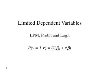
4. Probit Model (K.Train, Ch.5 ; Franses and Paap, Ch.4-5)
4. Probit Model • Based on the general RUM-model • Ass.: error terms are distributed normal with a mean vector of zero and covariance matrix • density function:
4. Probit Model Logit or Probit? • Trade-off between tractability and flexibility • Closed-form expression of the integral for Logit, not for Probit models • Probit allows for random taste variation, can capture any substitution pattern, allows for correlated error terms and unequal error variances Dependent on the specifics of the choice situation
4. Probit Model Estimation • Approximation of the multidimensional integral • Non-simulation procedures (see Kamakura 1989) Can usually only be applied to restricted cases and/or provide inaccurate estimations • Simulation procedures (see Geweke et al.1994, Train)
4. Probit Model Simulation-based estimation(binary probit, CFS) • Step 1 • For each observation n=1, ..., N draw r ~ N(0,1), (r = 1, ......., R: repetitions) • Initialize y_count= 0, =mt (starting values) • Compute y*rn = xn mt + L r ; L= choleski factor (LL’= ) • Evaluate: y*rn >0 y_count= y_count+1 • Repeat R times Weeks (1997)
4. Probit Model Simulation-based estimation(binary probit, CFS) • Step 2: calculate probabilities Pn| mt= y_count/R • Step 3: Form the simulated LL function SLL= n yn ln(Pn|mt)+(1-yn) ln(1-Pn|mt) • Step 4: Check convergence criteria (SLL(mt)- SLL(mt-1)) • Step 5: Update mt: mt+1 = mt + v • Step 6: Iterate (until convergence) Weeks (1997)
4. Probit Model Simulation-based estimation: MNProbit • Based on same principles • More efficient simulation procedures (see Train) • Identification: normalization of level and scale • Re-express model in utility differences • Normalization of varcov matrix (see Train)
4. Probit Model • Random taste variation • Model with random coefficients • E.g.: n~N(b,W) • Unj = b’xnj+ *’n xnj + nj • = b’xnj+ nj • nj : correlated error terms (dep.on xnj, see Train)
4. Probit Model • Substitution patterns • Full covariance matrix (no parameter restrictions) unrestricted substitution patterns • Structured covariance matrix (restrictions on some covariance parameters) • the structure imposed on determines the substitution pattern and may allow to reduce the number of parameters to be estimated
4. Probit Model • Example (Kamakura and Srivastava 1984): random utility components ni, nj are more (less) highly correlated when i and j are more (less) similar on important attributes (dij = weighted eucledian distance between i & j)
4. Probit Model • Examples • Choice models at brand-size level: correlation between ≠ sizes of same brand (Chintagunta 1992) MNL model gives biased estimates of price elasticity
4. Probit Model • Examples • Firm innovation (Harris et al. 2003) • Binary probit model for innovative status (innovation occurred or not) • Based on panel data correlation of innovative status over time: unobserved heterogeneity related to management ability and/or strategy
Model (2)-(4) account for unobserved heterogeneity (ρ) -> superior results
4. Probit Model • Examples • Dynamics of individual health (Contoyannis, Jones and Nigel 2004) • Binary probit model for health status (healthy or not) • Survey data for several years correlation over time (state dependence) + individual-specific (time-invariant) random coefficient
4. Probit Model • Examples • Choice of transportation mode (Linardakis and Dellaportas 2003) Non-IIA substitution patterns
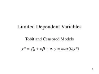
5. Ordered Logit Model • Choice between J>2 ordered ‘alternatives’ • Ordinal dependent variable y = 1, 2, ... J, with rank(1) < rank(2) < ... < rank(J) • Example: • Purchase of 1, 2, ... J units • Evaluation on a J-point scale ranging from, e.g., ‘dislike very much’ to ‘like very much’
5. Ordered Logit Model • Suppose yi* is a continous latent variable which • is a linear function of the explanatory variables yn* = Xn + n • and can be ‘mapped’ on an ordered multinomial variable as follows: yn= 1 if 0 < yn* 1 yn= j if j-1 < yn* j yn= J if J-1 < yn* J 0 < 1 < …. < j < … < J
5. Ordered Logit Model Ordered logit (see above) • 0 , J and 0: set equal to zero
5. Ordered Logit Model Interpretation of parameters (marginal effects)
5. Ordered Logit Model Estimation: ML
5. Ordered Logit Model • Disadvantages (Borooah 2002) • Assumption of equal slope k • Biased estimates if assumption of strictly ordered outcomes does not hold • treat outcomes as nonordered unless there are good reasons for imposing a ranking
5. Ordered Logit Model Example: Effectiveness of better public transit as a way to reduce automobile congestion and air polution in urban areas • Research objective: develop and estimate models to measure how public transit affects automobile ownership and miles driven. • Data: Nationwide Personal Transportation Survey (42.033 hh): socio-demo’s, automobile ownership and use, public transportation avail. Kim and Kim (2004)
5. Ordered Logit Model • Dependent variable ownership model = number of cars (k = 0, 1, 2, 3) ordinal variable • C*i = latent variable: automobile ownership propensity of hh i • Relation to observed automobile ownership: Ci=k if k-1 < ’xi + < k • P(Ci=k)=F(k- ’xi) - F(k-1 - ’xi) Kim and Kim (2004)
5. Ordered Logit Model • Examples • Occupational outcome as a function of socio-demographic characteristics (Borooah) • Unskilled/semiskilled • Skilled manual/non-manual • Professional/managerial/technical • School performance (Sawkins 2002) • Grade 1 to 5 • Function of school, teacher and student characteristics • Level of insurance coverage
D.Heterogeneity • Observed heterogeneity • Unobserved heterogeneity • Over decision makers • Random coefficients Models • E.g. Mixed Logit Model (see Train) • Over segments • Latent class estimation
D.Heterogeneity: Latent class est. • Ass.: Consumers can be placed into a small number of – homogeneous - segments which differ in choice behavior ( response parameters) • Relative size of the segment s (s=1, 2, ..., M) is given by fs = exp(s) / s’exp(s’) Kamakura and Russell (1989)