Download
1 / 35
420 likes | 1.11k Vues
JPEG Compression Algorithm In CUDA. Group Members: Pranit Patel Manisha Tatikonda Jeff Wong Jarek Marczewski Date: April 14, 2009. Outline. Motivation JPEG Algorithm Design Approach in CUDA Benchmark Conclusion. Motivation. Growth of Digital Imaging Applications

E N D
JPEG Compression Algorithm In CUDA Group Members: Pranit Patel ManishaTatikonda Jeff Wong JarekMarczewski Date: April 14, 2009
Outline • Motivation • JPEG Algorithm • Design Approach in CUDA • Benchmark • Conclusion
Motivation • Growth of Digital Imaging Applications • Effective algorithm for Video Compression Applications • Loss of Data Information must be minimal • JPEG • is a lossy compression algorithm that reduces the file size without affecting quality of image • It perceive the small changes in brightness more readily than we do small change in color
JPEG Algorithm • Step 1: Divide sample image into 8x8 blocks • Step 2: Apply DCT • DCT is applied to each block • It replaces actual color of block to average matrix which is analyze for entire matrix • This step does not compress the file • In general: Simple color space model: [R,G,B] per pixel JPEG uses [Y, Cb, Cr] Model Y = Brightness Cb = Color blueness Cr = Color redness
JPEG Algorithm • Step 3: Quantization • First Compression Step • Each DCT coefficient is divided by its corresponding constant in Quantization table and rounded off to nearest integer • The result of quantizing the DCT coefficients is that smaller, unimportant coefficients will be replaced by zeros and larger coefficients will lose precision. It is this rounding-off that causes a loss in image quality. • Step 4: Apply Huffman Encoding • Apply Huffman encoding to Quantized DCT Coefficient to reduce the image size further • Step 5: Decoder • Decoder of JPEG consist of: • Huffman Decoding • De-Quantization • IDCT
Discrete Cosine Transform • Separable transform algorithm (1D and then the 2D): • 2D DCT is performed in a 2 pass approach one for horizontal direction and one for vertical direction DCT 1st pass 2nd pass
Discrete Cosine Transform Translate DCT into matrix cross multiplication Pre-calculate Cosine values are stored as constant array Inverse DCT are calculated in the same way only with P00 P01 P02 P03 P04 P05 P06 P07 C00 C01 C02 C03 C04 C05 C06 C07 P10 P11 P12 P13 P14 P15 P16 P17 C10 C11 C12 C13 C14 C15 C16 C17 P20 P21 P22 P23 P24 P25 P26 P27 C20 C21 C22 C23 C24 C25 C26 C27 x P30 P31 P32 P33 P34 P35 P36 P37 C30 C31 C32 C33 C34 C35 C36 C37 P40 P41 P42 P43 P44 P45 P46 P47 C40 C41 C42 C43 C44 C45 C46 C47 P50 P51 P52 P53 P54 P55 P56 P57 C50 C51 C52 C53 C54 C55 C56 C57 P60 P61 P62 P63 P64 P65 P66 P67 C60 C61 C62 C63 C64 C65 C66 C67 P70 P71 P72 P73 P74 P75 P76 P77 C70 C71 C72 C73 C74 C75 C76 C77
DCT CUDA Implementation Each thread within each block has the same number of calculation Each thread multiply and accumulated eight elements P00 P01 P02 P03 P04 P05 P06 P07 C00 C01 C02 C03 C04 C05 C06 C07 P10 P11 P12 P13 P14 P15 P16 P17 C10 C11 C12 C13 C14 C15 C16 C17 P20 P21 P22 P23 P24 P25 P26 P27 C20 C21 C22 C23 C24 C25 C26 C27 x P30 P31 P32 P33 P34 P35 P36 P37 C30 C31 C32 C33 C34 C35 C36 C37 P40 P41 P42 P43 P44 P45 P46 P47 C40 C41 C42 C43 C44 C45 C46 C47 P50 P51 P52 P53 P54 P55 P56 P57 C50 C51 C52 C53 C54 C55 C56 C57 P60 P61 P62 P63 P64 P65 P66 P67 C60 C61 C62 C63 C64 C65 C66 C67 P70 P71 P72 P73 P74 P75 P76 P77 C70 C71 C72 C73 C74 C75 C76 C77 Thread.x = 2 Thread.y = 3
DCT Grid and Block Two methods and approach Each thread block process 1 macro blocks (64 threads) Each thread block process 8 macro blocks (512 threads)
DCT and IDCT GPU results 512x512 1024x768 2048x2048
Quantization Break the image into 8x8 blocks 8x8 Quantized matrix to be applied to the image. Every content of the image is multiplied by the Quantized value and divided again to round to the nearest integer value.
Quantization CUDA Programing Method 1 – Exact implementation as in CPU Method 2 – Shared memory to copy 8x8 image Method 3 – Load divided values into shared memory.
Tabulated Results for Quantization Method 2 and Method 3 have similar performance on small image sizes Method 3 might perform better on images bigger that 2048x2048 Quantization is ~x70 faster for the first method and much more as resolution increases. Quantization is ~ x180 faster for method2 and 3 and much more as resolution increases.
Huffman Encoding Basics • Utilizes frequency of each symbol • Lossless compression • Uses VARIABLE length code for each symbol IMAGE
Challenges • Encoding is a very very very serial process • Variable length of symbols is a problem • Encoding: don’t know when symbols needs to be written unless all other symbols are encoded. • Decoding: don’t know where symbols start
DECODING • Decoding: don’t know where symbols start • Need redundant calculation • Uses decoding table, rather then tree • Decode then shift by n bits. • STEP 1: • divide bitstream into overlapping segments. 65 bytes. • Run 8 threads on each segment with different starting positions
DECODING • STEP 2: • Determine which threads are valid, throw away others
DECODING - challenges • Each segment takes fixed number of encoded bits, but it results in variable length decoded output • 64 bit can result in 64 bytes of output. • Memory explosion • Memory address for input do not advance in fixed pattern as output address • Memory collisions • Decoding table doesn’t fit into one address line • Combining threads is serial • NOTE: to simplify the algorithm, max symbol length was assumed to be 8 bits. (it didn’t help much)
Huffman Results • Encoding • Step one is very fast: ~100 speed up • Step two – algorithm is wrong – no results • Decoding • 3 times slower then classic CPU method. • Using shared memory for encoding table resolved only some conflicts (5 x slower -> 4 x slower) • Conflicts on inputs bitstream • Either conflicts on input or output data • Moving 65 byte chunks to shared memory and ‘sharing’ it between 8 threads didn’t help much (4 x slower -> 3 x slower) • ENCODING should be left to CPU
Performance Gain DCT and IDCT are the major consumers of the computation time. Computation increases with the increase with resolution. Total Processing time for 2k image is 5.224ms and for the CPU is 189.59 => speed up of 36x
GPU Performance DCT and IDCT still take up the major computation cycles but reduced by a x100 magnitude. 2K resolution processing time is 7ms using the GPU as compared to ~900ms with the CPU.
Conclusion CUDA implementation for transform and quantization is much faster than CPU (x36 faster) Huffman Algorithm does not parallelize well and final results show x3 slower than CPU. GPU architecture is well optimized for image and video related processing. High Performance Applications - Interframe, HD resolution/Realtime video compression/decompression.