Download
1 / 25
250 likes | 360 Vues
High Resolution Imaging with Lasers. By Chris Krumm ECE401. Team. *Main Team *Christopher Krumm *Substantial Support Fernando Brizuela Courtney Brewer Senior Advisor: *Dr. Menoni. *Courtney and Fernando: underlying theory and providing feedback *Dr. Menoni: goals and guidance

E N D
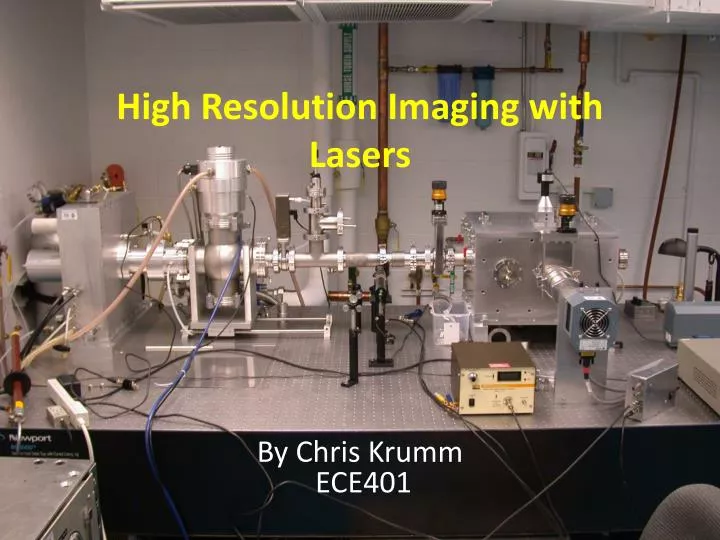
High Resolution Imaging with Lasers By Chris Krumm ECE401
Team *Main Team *Christopher Krumm *Substantial Support Fernando Brizuela Courtney Brewer Senior Advisor: *Dr. Menoni
*Courtney and Fernando: underlying theory and providing feedback *Dr. Menoni: goals and guidance *Courtney and Fernando also: demonstrated the microscope last summer; obtained experimental results
Budget Personally: • No personal purchases other than labor (time) System: • Synchrotron construction and operation will cost on the order of hundreds of millions vs. • One of our recent laser systems ran for 180 thousand dollars producing in the EUV spectrum
Applications and Future Work • Nanoscale (sub 100nm) imaging, (nanotubes, Nanoparticles, Small Features) • Niche applications unsuitable for Customers…. Governments, corporations, laboratories wanting imaging on the sub 100nm regime My work would affect interpretation of the limits of our resolution, greater understanding, affects of diffraction on images, compare with other software (the code is not available and we know there are problems) for bet
function CCSplat8 • %addpath('U:\ERC\CCSplat') %copy into workspace to begin program • %addpath('C:\Documents and Settings\Christopher\Desktop\CCSplat') • %addpath('C:\Documents and Settings\Christopher\Desktop\SRDesignFinal Report') • %addpath('U:\ERC'); • %variables: • %Imo = object matrix, p = pupil function matrix • %C and D are specialized integer matrices for the phase factor • %lambda .... d0 is object to pupil distance, d1 pupil to image distance • m = 10^(0); • cm = 10^(-2); • mm = 10^(-3); • um = 10^(-6); • nm = 10^(-9); • pm = 10^(-12); • fm = 10^(-15); • lambda = 46.9*nm; • k=2*3.14159265/lambda;
d0 = 1.2*mm; %propagation distance object to lense (ZP) • d1 = 1; %propagation distance lense to imaging screen • Imo = ones(1024,1024); %set this matrix with ones • u = -512:511; %generate 1,2,3,4,5...1023,1024 • j = u.^2; %square the last entries: 1,4,9... • C = repmat(j,1024,1); %so that A is for phase term inside • D = transpose(C); %this automatically sets matrix B up so • Imo = 1-Imo; %so x is now all zeros • %%for square • %for (i = 1:512); • % for (j = 1:512); %this is grating thickness • % %for square: Imo(i+512-16,j+512-16)=1; • % Imo(i+256,j+256)=1; • % end; • %end; • %for grating: • for (stripe = 1:8); • for (i = 1:60); • for (j = 1:200); %this is grating thickness • %for square: Imo(i+512,j+512)=1; • %Imo(stripe*100+i+100,j+512)=1; • Imo(stripe*120+i-60,j+406)=1; • end; • end; • end; • vx = 1:1:1024;%vector to scale x axis on plot • vy = 1:1:1024;%vector to scale y axis on plot
figure(1); • subplot(2,3,1); • imagesc(vx,vy,Imo); %figuresub#1 is the Object plot • title('Object Plot'); • axis square • xlabel('nm'); • ylabel('nm'); • %------------------------------------------------------------ • %for making a circle: • p = zeros(1024,1024); • for(j =-9:9); • for(i=floor(-sqrt(9^2-j.^2)):floor(sqrt(9^2-j.^2))); %%note jmax • p(j+512,i+512)=1; %%note j+delta, i+delta has delta as matrix length over 2 • end; • end • figure(1); • subplot(2,3,2); • imagesc(p); %figuresub#2 is the pupil function plot • title('Pupil Plot'); • axis square • xlabel('23um'); • ylabel('23um');
%------------------------------------------------------------%------------------------------------------------------------ • figure(2); • imagesc(abs(fftshift(fft2(p)))); • axis square • title('linear impulse response'); • xlabel('46.9nm*1m/(1024(23um))'); • ylabel('46.9nm*1m/(1024(23um))'); • %------------------------------------------------------------ • Hp = (fftshift(fft2((fft2(p))))); %this sets up fourier transform of impulse response. • %plots the transform (of the impulse response) • figure(1); • subplot(2,3,3); • imagesc(abs(fftshift(Hp))); • axis square • title('Double Transform of Pupil Function'); • xlabel('46.9nm*1mm/(2*1024nm)=23um'); • ylabel('46.9nm*1mm/(2*1024nm)=23um'); • Gi = (fft2(Imo)); %this sets up the fourier transform of the object • %plots the object's frequency at the pupil function • figure(1); • subplot(2,3,4); • imagesc(abs(fftshift(Gi))); • axis square • title('Object linear frequency domain'); • xlabel('nm'); • ylabel('nm');
size(Gi) • size(Hp) • Ifmo = Gi.*Hp; %multiplies transforms together • %plot the product of frequencies • figure(1); • subplot(2,3,5); • imagesc(abs(fftshift(Ifmo))); • axis square • title('Linear Frequency Product'); • xlabel('23um'); • ylabel('23um'); • Imi = ((ifft2((Ifmo)))); %sets up an image based on the inverse transforms • %plot tthe image • figure(1); • subplot(2,3,6); • imagesc(abs(Imi)); • axis square • title('Image'); • xlabel('nm*1000'); • ylabel('nm*1000');
%____________________________________________________________________%____________________________________________________________________ • %____________________________________________________________________ • %____________________________________________________________________ • %Now for the fresnel propagator: note that the matrices for pupil functin • %and object have to be entered with the appropriate ratios; the object • %must be sized appropriately. The two matrices have the same • %units (micrometers per pixel are the same for each matrix). • %The fourier transform of the object is then • % propagated to the lense plane and in my program is DIRECTLY • %multiplied by the pupil function; this product is then • %propagated to the imaging plane/screen. • %DIRECTLY BELOW IS THE FRESNEL PROPAGATOR CODE • y2 = Imo.*exp(sqrt(-1)*k/(2*d0).*(C+D).*(1*nm)^2); %this inserts the quadratic phase factor • %plot the object (times phase factor should be same) • figure(3); • subplot(2,3,1); • imagesc(abs(y2)); • axis square • title('Image object'); • xlabel('nm'); • ylabel('nm'); • %plot the pupil function as reminder • figure(3); • subplot(2,3,2); • imagesc(abs(p)); • axis square • title('Pupil Function'); • xlabel('23um'); • ylabel('23um');
%plot the object propagated to pupil plane: • figure(3); • subplot(2,3,3); • imagesc(fftshift(abs(fft2(y2)))); • axis square • title('Object propagated to pupil plane'); • xlabel('23um'); • ylabel('23um'); • %plot all products together at the pupil plane • fft1er = fftshift(fft2(y2)).*p.*exp(-sqrt(-1)*k/(2*(1/d0+1/d1)).*(C+D).*(20*um)^2); %direct multiplication of fft of y2 with pupil function • %note that f = 1/d0+1/d1 • figure(3); • subplot(2,3,4); • imagesc(abs(fft2(fft1er))); • axis square • title('Product at pupil plane'); • xlabel('23um'); • ylabel('23um');
freqmulti2 = fft1er.*exp(sqrt(-1)*2*3.14159265/lambda/(2*d1).*(C+D).*(20*um)^2); • %don't need to plot freqmulti as it will be the same as the products before • ImagePlane = fft2(freqmulti2); • %plot the image • figure(3); • subplot(2,3,5); • imagesc(abs((ImagePlane))); • axis square • title('Image'); • xlabel('nm*1000'); • ylabel('nm*1000'); • %Before was the linear case, no need to worry about magnification because • %so far the user must enterpret the values entered into the program and the • %magnification of the system based on the distance ratio d1/d0 • end
Future Goals • Extend to the incoherent case of radiation • Prepare direct cut outs of the modulation transfer function and compare with experiment • Extend to higher pixels (allocate more memory to Matlab, go to 4096 pixels, modify to include reflection mode (perhaps look at distortion due to change in focus)) • Analyze different samples • Analyz the partially coherent case directly
*ignoring the 2nd order effects *Best Zone Plate (70nm) *50nm half period grating
Including 2nd Order Effects: Notice that we seem to be missing a fringe with 2nd order effects, also notice that displacement is affected more when the object is not centered with the zone plate.
*Including the 2nd order effects *Best Zone Plate (70nm) *60nm half period grating • My simulation predicts faster modulation rise with grating size
Conclusions • My simulation seems to be predicting accurately the limit of resolution for each zone plate, along with effects that we observed last summer imaging gratings.