Download
1 / 25
250 likes | 375 Vues
Keldysh Model in Time Domain. K onstantin Kikoin ( Tel-Aviv University ) M ichael Kiselev ( ICTP, Trieste ). Motivation : TLS is as universal as an oscillator . We will play with TLS ensemble in order to extend to time domain

E N D
Keldysh Model in Time Domain Konstantin Kikoin (Tel-Aviv University) Michael Kiselev (ICTP, Trieste)
Motivation:TLS is as universal as an oscillator. • We will play with TLS ensemble in order to extend to time domain • exactly solvable Keldysh model originally invented for description of • disordered semiconductors (L.V.Keldysh ‘65) developed by A.Efros(’71) • and exploited by M.V.Sadovskii (’74,’79 ff),Bartosh&Kopietz (’00) etc • Applications: • Time dependent Landau-Zener problem • Well population redistribution in optical lattices • Tunneling through quantum dots in presence of noise Publications: JETP Letters 89, 133 (2009); arXiv:0901.2246 arXiv:0803.2676; Phys. Stat. Solidi (c) (in press)
Time-dependent Landau-Zener model(Kayanuma ’84-85) The source of temporal fluctuations is the phonon bath
Optical lattice in random laser field 3D tetragonal optical lattice with split traps ( PRL ‘08) Fluctuations φ(t) may be the source of noise
Double-well quantum dot with time-dependent gate voltage DQD “Which pass” geometry s T-shape geometry W Vgt) s d δ(t) Electron possesses both spin ½ and pseudospin ½ corresponding to two positions in DQD. The symmetry of this objects is SU(4) ∆(t) d
ORIGINAL KELDYSH MODEL KM was proposed for description of non-interacting electrons in a random potential V(r) (disordered electrons in metals or semiconductors) G(r,r’) – bare electron propagator (cross technique) Vertex corrections Self energy corrections
Usual approach - white noise (Gaussian) approximation Short-range δ-like scattering Keldysh model (“anti- white noise”) - infinite-range scattering Impurity field is constant in each realization, but its magnitude changes randomly from one realization to another. The perturbation series for the Green function can be summed exactly in approximation of IRS because all cross diagrams in a given order are equivalent
An is the total number of diagrams in the order 2n – purely combinatorial coefficient, Then Keldysh uses the integral representation and changes the order of summation and integration (Borel summation procedure) Summation results in Gaussian distribution for GR This means that an electron moves in a spatially homogeneous field V, and the magnitude of this field obeys the Gaussian distribution with the variance W Our idea is to convert the Keldysh model into the time domain
Time-Dependent Keldysh Model (TDKM) Random field V(t) fluctuating in time: (t2) (t2) (t3) Then one may apply cross technique and Keldysh machinery to the ensemble of TLS, Now disorder develops on the 1D time axis instead of spatial lattice or chain. We apply this model to an ensemble of TLS consisting either of fermions or of bosons
Wide barrier limit: l– spin up, r – spin down leftright Original Hamiltonian (Fermi/Bose-Hubbard model): Effective Hamiltonian for N = 1 rewritten in terms of Pauli matrices for two states {l,r} symmetric “Lifshitz’ ass” asymmetric δ0 Both Δ and δ may slowly fluctuate in time
Time-dependent random fluctuations of asymmetry parameter: The analog of Keldysh conjecture: slowly varying random field ~ exp(- γt) . Then the Fourier transform of the noise correlation function is This means that we consider the ensemble of states with a field δ = constin a given state, but this constant is random in each realization . Then we apply the cross technique in time domain to the single particle propagator
are the bare propagators for a particle in the left and right valley. Repeating Keldysh’ calculations, we obtain The same for Gr,s(ε+ δ0) . Remarkably, the Green function after Gaussian averaginig has no poles, singularities or branch cuts.
“Vector” Keldysh model for fluctuating transparency Δ Let us considersymmetric TLS with nearly impenetrable barrier ∆0 → 0 and allow intervalley tunneling only due to the random transverse perturbation and make Keldysh conjecture about correlation function namely, approximate its Fourier transform by Now the cross technique is subject to kinematic restriction. Each site is associated ether with σ+ or with σ- but and only diagrams with pseudospin operators ordered as
As a result the series becomes two-colored: and the dashed lines connect only vertices of different colors Keldysh summation is still possible but the combinatorial coefficients differ from those in “scalar” model with Similar expansion for “vector Keldysh model in real space was obtained by Sadovskii (’74) in a model of long-range fluctuations near the CDW instability.
Again we use the integral representation and perform Borel summation. The result: Two-dimensional Gaussian averaging of vector random field with transversal (xy) fluctuations. Like in the scalar Keldysh model, the Green functions have no poles. This means that the information about position of the particle in the left or right valley is partially lost due to stochastization.
More general result by simpler method(path integral formalism) Lagrangian action:
Green function in a symmetric TLS From “Bloch ellipsoid” to “Bloch sphere”: Turning to spherical cordinates and integrating over angles, we have Ellipsoid transforms into sphere for ζ= ξ Scalar model: ξ→0 Planar model: ζ→ 0
Density of States in stochastisized TLS Scalar TDKM: two superimposed Gaussians Planar TDKM: single Gaussian with pseudogap around zero energy (cf. Sadovskii ) What about experimental manifestations?
What is already seen in optical lattice with split potental wells? Repopulation of these wells |n, m > → |n-1, m+1>
What we propose: resulting in noise-induced mixed valence states of the split optical trap
s TDKM for Double Quantum Dots Vg(t) d N=1:Pseudospin is screened but spin survives: Noise induced “local phase transition” SU(4) → SU(2) In more refinedmodels with SO(5) symmetry spin degrees of freedom also may be dynamically stochastisized (K.K., M.K. and J. Richert ,‘08, ’09)
Conclusions • Keldysh model looks more realistic in time domain (long memory) • than in real space (infinite range correlations) • TDQM is useful in study of decoherence effects in nanosystems • described in terms of TLS cells, including memory cells for quantum • computers
The spin susceptibility of stochastisized TLS or QD may be calculated in a very elegant way via “Ward identities” (Efros’71; K.K & K.M. ‘08) Direct differentiation of GF in Gaussian representation derived above shows that these GF obey differential equations for scalar TDKM (Efros) for vector TDKM (K.K & K.M) Now we may introduce the vertex parts Г using the analogy with Ward identities
First vertex corrections for scalar and vector TDKM. But these corrections may be found exactly by means of Ward identity WI reads ζ G2Г = εG - 1 with asymptotical behavior Thus spin is indeed stochastisized at low temperature !