Hough Transform and RANSAC

1. Hough Transform and RANSAC Various slides from previous courses by: D.A. Forsyth (Berkeley / UIUC), I. Kokkinos (Ecole Centrale / UCL). S. Lazebnik (UNC / UIUC), S. Seitz (MSR / Facebook), J. Hays (Brown / Georgia Tech), A. Berg (Stony Brook / UNC), D. Samaras (Stony Brook) . J. M. Frahm (UNC), V. Ordonez (UVA).

2. Last Class • Interest Points (DoG extrema operator) • SIFT Feature descriptor • Feature matching

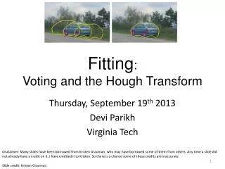
3. Today’s Class • Line Detection using the Hough Transform • Least Squares / Hough Transform / RANSAC

4. Line Detection Pixels in input image • Have you encountered this problem before?

5. Line Detection – Least Squares Regression Pixels in input image • Have you encountered this problem before? Find betas that minimize: Solution:

6. However Least Squares is not Ideal under Outliers Pixels in input image

7. Solution: Voting schemes • Let each feature vote for all the models that are compatible with it • Hopefully the noise features will not vote consistently for any single model • Missing data doesn’t matter as long as there are enough features remaining to agree on a good model Slides by Svetlana Lazebnik

8. Hough transform • An early type of voting scheme • General outline: • Discretize parameter space into bins • For each feature point in the image, put a vote in every bin in the parameter space that could have generated this point • Find bins that have the most votes Image space Hough parameter space P.V.C. Hough, Machine Analysis of Bubble Chamber Pictures, Proc. Int. Conf. High Energy Accelerators and Instrumentation, 1959 Slides by Svetlana Lazebnik

9. Parameter space representation • A line in the image corresponds to a point in Hough space Image space Hough parameter space Source: S. Seitz

10. Parameter space representation • What does a point (x0, y0) in the image space map to in the Hough space? Image space Hough parameter space

11. Parameter space representation • What does a point (x0, y0) in the image space map to in the Hough space? • Answer: the solutions of b = –x0m + y0 • This is a line in Hough space Image space Hough parameter space

12. Parameter space representation • Where is the line that contains both (x0, y0) and (x1, y1)? Image space Hough parameter space (x1, y1) (x0, y0) b = –x1m + y1

13. Parameter space representation • Where is the line that contains both (x0, y0) and (x1, y1)? • It is the intersection of the lines b = –x0m + y0 and b = –x1m + y1 Image space Hough parameter space (x1, y1) (x0, y0) b = –x1m + y1

14. Parameter space representation • Problems with the (m,b) space: • Unbounded parameter domains • Vertical lines require infinite m

15. Parameter space representation • Problems with the (m,b) space: • Unbounded parameter domains • Vertical lines require infinite m • Alternative: polar representation Each point (x,y) will add a sinusoid in the (,) parameter space

16. Algorithm outline • Initialize accumulator H to all zeros • For each feature point (x,y) in the image For θ = 0 to 180ρ = x cos θ + y sin θ H(θ, ρ) = H(θ, ρ) + 1 endend • Find the value(s) of (θ, ρ) where H(θ, ρ) is a local maximum • The detected line in the image is given by ρ = x cos θ + y sin θ ρ θ Slide by Svetlana Lazebnik

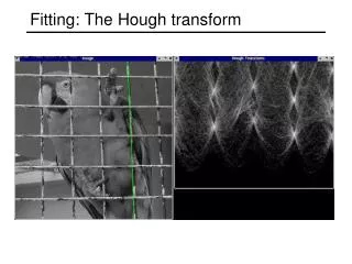
17. Basic illustration votes features

18. Hough Transform for an Actual Image

19. Edges using threshold on Sobel’s magnitude

20. Hough Transform (High Resolution)

21. Hough Transform (After threshold)

22. Hough Transform (After threshold) Vertical lines

23. Hough Transform (After threshold) Vertical lines

24. Hough Transform with Non-max Suppression

25. Back to Image Space – with lines detected

26. Hough transform demo

27. Incorporating image gradients • Recall: when we detect an edge point, we also know its gradient direction • But this means that the line is uniquely determined! • Modified Hough transform: • For each edge point (x,y) θ = gradient orientation at (x,y)ρ = x cos θ + y sin θ H(θ, ρ) = H(θ, ρ) + 1end Slide by Svetlana Lazebnik

28. Hough transform for circles image space Hough parameter space r y (x,y) x x y Slide by Svetlana Lazebnik

29. r x y Hough transform for circles • Conceptually equivalent procedure: for each (x,y,r), draw the corresponding circle in the image and compute its “support” Is this more or less efficient than voting with features? Slide by Svetlana Lazebnik

30. RANSAC – Random Sample Consensus • Another Voting Scheme • Idea: Maybe you do not need to have all samples have a vote. • Only a random subset of samples (points) vote.

31. visual codeword withdisplacement vectors training image Generalized Hough Transform • You can make voting work for any type of shape / geometrical configuration. Even irregular ones. B. Leibe, A. Leonardis, and B. Schiele, Combined Object Categorization and Segmentation with an Implicit Shape Model, ECCV Workshop on Statistical Learning in Computer Vision 2004

32. Generalized Hough Transform • You can make voting work for any type of shape / geometrical configuration. Even irregular ones. B. Leibe, A. Leonardis, and B. Schiele, Combined Object Categorization and Segmentation with an Implicit Shape Model, ECCV Workshop on Statistical Learning in Computer Vision 2004 test image

33. RANSAC (RANdom SAmple Consensus) : Fischler & Bolles in ‘81. • Algorithm: • Sample (randomly) the number of points required to fit the model • Solve for model parameters using samples • Score by the fraction of inliers within a preset threshold of the model • Repeat 1-3 until the best model is found with high confidence

34. RANSAC Line fitting example • Algorithm: • Sample (randomly) the number of points required to fit the model (#=2) • Solve for model parameters using samples • Score by the fraction of inliers within a preset threshold of the model • Repeat 1-3 until the best model is found with high confidence Illustration by Savarese

35. RANSAC Line fitting example • Algorithm: • Sample (randomly) the number of points required to fit the model (#=2) • Solve for model parameters using samples • Score by the fraction of inliers within a preset threshold of the model • Repeat 1-3 until the best model is found with high confidence

36. RANSAC Line fitting example • Algorithm: • Sample (randomly) the number of points required to fit the model (#=2) • Solve for model parameters using samples • Score by the fraction of inliers within a preset threshold of the model • Repeat 1-3 until the best model is found with high confidence

37. RANSAC • Algorithm: • Sample (randomly) the number of points required to fit the model (#=2) • Solve for model parameters using samples • Score by the fraction of inliers within a preset threshold of the model • Repeat 1-3 until the best model is found with high confidence

38. How to choose parameters? • Number of samples N • Choose N so that, with probability p, at least one random sample is free from outliers (e.g. p=0.99) (outlier ratio: e ) • Number of sampled points s • Minimum number needed to fit the model • Distance threshold  • Choose  so that a good point with noise is likely (e.g., prob=0.95) within threshold • Zero-mean Gaussian noise with std. dev. σ: t2=3.84σ2 For p = 0.99 modified from M. Pollefeys

39. RANSAC conclusions Good • Robust to outliers • Applicable for larger number of model parameters than Hough transform • Optimization parameters are easier to choose than Hough transform Bad • Computational time grows quickly with fraction of outliers and number of parameters • Not good for getting multiple fits Common applications • Computing a homography (e.g., image stitching) • Estimating fundamental matrix (relating two views)

40. How do we fit the best alignment? How many points do you need?

41. Questions?