Download
1 / 1
10 likes | 177 Vues
Y. X. T. B. X. 4. 1. 8. 5. 0. Time (ms). 3000. Frame 1. Frame 2. Frame 3. Time. C. D. E. Mode1 Vs. Sum of All modes. Mode2 Vs. Sum of All modes. Actual gut motion Vs. Sum of All modes. A. B. Modes.

E N D
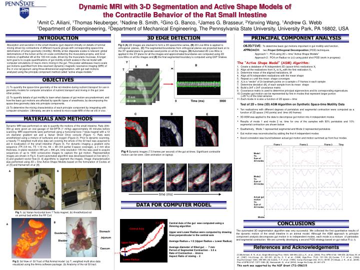
Y X T B X 4 1 8 5 0 Time (ms) 3000 Frame 1 Frame 2 Frame 3 Time C D E Mode1 Vs. Sum of All modes Mode2 Vs. Sum of All modes Actual gut motion Vs. Sum of All modes A B Modes Fig 1: (a) Varian horizontal bore 7 Tesla magnet. (b) Anesthetized rat on animal bed within the RF Coil. b B A Stomach Duodenum Jejunum Bladder Caecum Fig 2: 3d View of GI Tract of Rat Animal model :(a) T1 weighted multi slice data visualized using the Amira software package. (b) Anatomy of the rat GI tract. Dynamic MRI with 3-D Segmentation and Active Shape Models of the Contractile Behavior of the Rat Small Intestine 1Amit C. Ailiani, 1Thomas Neuberger, 1Nadine B. Smith, 2Gino G. Banco, 2James G. Brasseur, 2Yanxing Wang, 1Andrew G. Webb 1Department of Bioengineering, 2Department of Mechanical Engineering, The Pennsylvania State University, University Park, PA 16802, USA INTRODUCTION 3D EDGE DETECTION PRINCIPAL COMPONENT ANALYSIS Absorption and secretion in the small intestine (gut) depend critically on details of luminal mixing driven by contractions of different muscle groups with corresponding space-time deformation of lumen geometry (motility). Motility at two disparate scales is relevant: global deformations of the lumen at the cm scale controlled by the muscularis propria, and local motions of epithelial villi at the 100 mm scale, driven by the muscularis mucosae. A longer term goal is to couple quantifications of gut motility at both scales in the rat model with computer simulations of macro-micro mixing in the gut. This poster addresses macro-scale gut motions quantified from time-resolved (dynamic) magnetic resonance imaging (MRI) of the in vivo rat jejunum using three-dimensional segmentation, with gut wall motions analyzed using the principle component method called “active shape models.” Fig 3 (A) 2D Images are stacked to form a 3D space/time series, (B) 2D Live-Wire is applied to orthogonal planes, (C) The segmented boundaries from orthogonal planes are projected back on to the XY spatial plane to generate seed points on all the images, (D) Automated 2D Live-Wire is applied in the XY plane for all the images and approximated boundaries are computed using 2D Live-Wire on all the images and (E) the final segmented boundary is computed using GVF Snakes. OBJECTIVE: To determine basic gut motions important in gut motility and function. APPROACH: two Proper Orthogonal Decomposition (POD) techniques. Approach 1 :PCA using 2D + time “Active Shape Models” Approach 2: PCA on Radius vs (z,t) using pistol shot POD (work in progress) The “Active Shape Model” (ASM) Algorithm: • Create a database of N independent 3D (space-time) realizations Xt • Align all the realizations from X2 to XN with the first realization X1 • Determine mean of the aligned realizations, M • Align all N independent realizations with the mean shape • Repeat a-c until the mean shape converges • Xtis a “vector” of 2n landmark points on a sample x F frames in each sample • Determine deviation dXt of each sample from its mean shape • Build a 2nF x 2nF covariance matrix • Covariance matrix is used to determine principal eigenvectors and its corresponding eigenvalues. • Complex gut motion can be represented by first m modes that represent larger portion (>95 %) of the total variance • Each mode m is also a function of 2D space + time A OBJECTIVES (1) To quantify the space-time geometry of the rat intestine during nutrient transport for use in geometry models for computer simulation of nutrient transport and mixing in the gut (see other poster). (2) To quantify details of gut motility to learn what classes of gut motion are predominant, and how the basic gut motions are affected by specific types of anesthesia, by decomposing the space-time geometry data into principle components. (3) To determine the mixing characteristics of each principle component by integrating with computer simulation. Ultimately, we aim to extend to micro-scale MRI of the rat villi in vivo. Test of 2D + time (3D) ASM Algorithm on Synthetic Space-time Motility Data • Ten realizations with different degrees of peristalsis and segmental contraction were computed as a function of 2D space (140 points) and time (40 frames) • 3D ASM was applied to the data to decompose gut motion into 4 independent modes • Results of mode 1 and mode 2 vs. time for one of the samples with 90% peristalsis and 10% segmental contraction are shown below • Qualitatively, Mode 1 represented segmental and Mode 2 represented peristalsis • Gut motion was reconstructed by adding the first 4 independent modes • Good correlation was found between actual gut motion and motion summed up from four modes MATERIALS AND METHODS Dynamic MRI was performed on rats to quantify the motions of the small intestine. Rats (200-300 g) were given an oral gavage of Gd-DPTA (1 ml/kg) approximately 45 minutes before scanning. MRI experiments were performed using a horizontal bore 7 tesla magnet with a 12 cm diameter gradient set and a Varian Direct Drive console (Figure 1). Rats were anesthetized using a mixture of isoflurane and oxygen (Figure 2). Prior to dynamic scanning, a heavily T1-weighted multi-slice data set covering the whole of the GI tract was acquired to aid in localization of the small intestine (Figure 3). For dynamic imaging a gradient echo sequence (TR 2.8 ms, TE 1.12 ms, 64 × 48 (3/4 partial k-space coverage), a 2 mm slice thickness, in-plane resolution 390 μm × 390 μm, time resolution 135 ms) was used to acquire sequences of up to 1000 consecutive images to capture the gut motion. Representative images are shown in Fig 4. A semi-automated algorithm was developed based on live-wire [1, 2] and gradient vector flow [3, 4] algorithms to segment the images. Image characterization was performed using 2D + time Active Shape Models based on the formulation of Cootes et al. [5]and Hamarneh et al. [8]. Fig 4 Dynamic images (7.5 frames per second) of the gut at times. Significant contractile motion can be seen. (See animation on laptop) time (ms) DATA FOR COMPUTER MODEL CONCLUSIONS z = 200 Central Axis of the gut was computed using a thinning algorithm Upper and Lower Radius were computed by drawing lines perpendicular to the central axis Average Radius = 1/2 (Upper Radius + Lower Radius) Average diameter of filled gut ~ 7 mm Period of Segmental Contraction ~ 3.5 s Rate of Contraction ~ 2mm/s Aspect Ratio of mixing ~ 2 Central Axis The automated 3D segmentation algorithm was very successful. We collected the first quantitative results of the dynamic motion of the small intestine in an animal model. Although the ASM approach to principle component analysis decomposes gut motion in to independent modes, each mode is a mixture of peristalsis and segmental contraction. We are currently developing a second POD strategy based on gut radius R (z, t). Upper Radius References and Acknowledgements z = 0 [1] Mortensen, E. N, et al., Graph.Mod.Imag.Proc. 60(5): 349-384, [2] Lu, K., et al., (2006). Proc SPIE 6144: 189-203. [3] Kass, M, et al., (1987). Int.J.Comp. (4): 321-331, [4] Xu, C. Y, et al., (1998). Sign.Proc. 71(2): 131-139. [5] Cootes, T. F, et al., (1994). Img.Vis.Comput 12(6): 355-365, [6] Cootes, T. F, et al., (1995). Comp.Vis.Image.Und. 61(1): 38-59. [7] Udupa, J. K., et al., (2005). Proc of SPIE 5747: 1377-1383. [8] Hamaraneh, G, et al. (2004). Image.Vis.Comp. 22: 461-470 This work was supported by the NSF Grant CTS-056215 Lower Radius