Download
1 / 22
220 likes | 383 Vues
Monitoring Air Quality Changes in Regions Influenced by Major Point Sources over the Eastern and Central United States Using Aura/OMI NO 2. Ken Pickering NASA Goddard Space Flight Center, Greenbelt, MD Ana Prados UMBC/JCET Goddard Space Flight Center, Greenbelt, MD

E N D
Monitoring Air Quality Changes in Regions Influenced by Major Point Sources over the Eastern and Central United States Using Aura/OMI NO2 Ken Pickering NASA Goddard Space Flight Center, Greenbelt, MD Ana Prados UMBC/JCET Goddard Space Flight Center, Greenbelt, MD Sergey NapelenokUS EPA, Research Triangle Park, NC
Introduction • Tropospheric NO2 observations from space : GOME 8/95-6/03 40 x 320 km* 10:30 AM LT SCIAMACHY 8/03 60 x 30 km** 10:00 AM LT OMI 11/04 13 X 24 km*** 1:30 PM LT GOME-2 3/07 40 X 80 km 9:30 AM LT * Global coverage in 3 days; **complete coverage at Equator in 6 days; ***nadir resolution, increasing to 40 X 160 km at edges • Trend analyses – examples: Richter et al. (2005): GOME and SCIAMACHY data used to show NO2 increases over China and decreases in US and Europe Kim et al. (2006): SCIAMACHY data used to demonstrate initial NO2 decrease due to SIP Call power plant emission reduction
2-dimensional CCD wavelength ~ 780 pixels ~ 580 pixels viewing angle ± 57 deg flight direction » 7 km/sec 13 km (~2 sec flight)) 2600km 13 km x 24 km (binned & co-added) Aura/OMI Ozone Monitoring Instrument Aura Wavelength range: 270 – 500 nm Sun-synchronous polar orbit; Equator crossing at 1:30 PM LT 2600-km wide swath; horiz. res. 13 x 24 km at nadir Global coverage every day O3, NO2, SO2, HCHO, aerosol, BrO, OClO
What has happened to Eastern US NOx emissions since 2002? • US EPA mandated power plant NOx emission reductions under the 1998 NOxState Implementation Plan Call. Nearly 40% reductions between 2002 and 2005 were documented by Kim et al. (2006) using SCIAMACHY NO2 data. • Program evolved into the “NOx Budget Trading Program”. Resulted in further summertime power plant emission reductions over the regulated region (19 eastern states), but trading program allows flexibility concerning the magnitude of reduction at specific facilities. • Clean Air Interstate Rule (CAIR) – resulted in further reductions (28 states), but rule thrown out by courts; then reinstated. Some companies reduced emissions in response to more stringent state rules and court orders. • Cross-State Air Pollution Rule (CSAPR) – announced July 2011; replaces CAIR; ozone season NOx reductions of 54% from 2005 required over 20 states by 2012.
July 2008 vs. July 2005 OMI Trop. NO2 -- % change Continuous Emission Monitoring System (CEMS) -- Absolute Changes
OMI NO2 Trend Calculation • Total NO2 and the NO2 sensitivity to NOx emissions from major point sources in selected regions at each model layer computed by CMAQ-DDM-3D • CMAQ tropospheric columns of total NO2 and the NO2 contribution from major point sources were calculated daily for OMI overpass time • The monthly mean fraction of the total CMAQ NO2 column contributed by these point sources was calculated for each model column • OMI tropospheric NO2 (0.05 degree Level 3 product) was regridded onto the CMAQ 12 km grid • The CMAQ columns corresponding to three fraction thresholds, 0.3, 0.4, and 0.6 were selected • For each month and year, the corresponding OMI NO2 regridded values were averaged into monthly means • OMI NO2 trends were calculated as the differences between the monthly means for each year (2006, 07, 08) and the 2005 means
CEMS Trend Calculation • CEMS point source NOxemissions were mapped onto the OMI NO2 grid, and monthly values (in tons/month) were calculated for the 2005-2008 time period • The trends were calculated as the difference between monthly NOx emissions from all grid cells contained within each selected region and the 2005 monthly emissions.
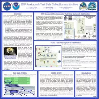
Decoupled Direct Method in 3D (DDM-3D) in CMAQ(Napelenok et al., 2008,Environ. Modeling and Software) Provides a measure of the change in pollutant concentrations due to changes in some parameter of interest (in this case emissions). Change in concentrations of specie i due to changes in emissions of j. DDM-3D provides sensitivity of gaseous pollutants (NO, NO2, O3, etc.) due to EGU emissions of NOx in 8 predefined geographical areas. MN WPAEOH LOHV MDSPA WMOEKS NEOK NGANAL NETXWLA
Application of CMAQ-DDM-3D in Trend Analysis • Ideally, one would want to run CMAQ-DDM-3D for the beginning year and end year of the trend period, and compute the OMI NO2 trend only for CMAQ grid cells with similar sensitivities in both years. • In this preliminary work we have a 2005 CMAQ-DDM-3D run and examine the monthly mean analyzed winds to determine similarities in transport between 2005 and 2008.
Example: August 2005 vs. 2008 GSFC/GMAO MERRA Winds U August 2005 U August 2008 V August 2005 V August 2008
Percentage Changes 2005 to 2008 NE TX – W LA June July Aug OMI trend in grid -29.2 -8.4 -16.6 cells with sensitivity ratio >0.6 CEMS trend -22.7 -15.6 -12.1 --------------------------------------------------------------------------------------------------------------- MN OMI trend in grid -34.3 -4.0 -25.5 cells with sensitivity ratio >0.6 CEMS trend -42.5 -23.8 -29.7 --------------------------------------------------------------------------------------------------------------- Moderate emission reductions in all three months; OMI trends similar Large emission reductions in all three months; OMI trends nearly as large except for July
Percentage Change 2005 to 2008 Large emission reductions in all three months; OMI shows small decrease in June, moderate in July, and decrease equal to CEMS in August. Other sources must have increased. Will need to compare 2005 and 2008 NEI. MD – S PA June July Aug OMI trend in grid -2.4 -13.5 -50.1 cells with sensitivity ratio >0.6 CEMS trend -34.6 -41.4 -49.6 ------------------------------------------------------------------------------------------------------------------- W MO – E KS OMI trend in grid -37.6 -31.3 -17.4 cells with sensitivity ratio >0.6 CEMS trend -41.6 -39.7 -35.1 ------------------------------------------------------------------------------------------------------------------- Large emission reductions in all three months; OMI shows nearly similar reductions except in August.
Percentage Change 2005 to 2008 Lower OH Valley June July Aug OMI trend in grid -25.4 -4.5 -23.7 cells with sensitivity ratio >0.6 CEMS trend +2.4 +6.2 +2.6 --------------------------------------------------------------------------------------------------------------- NE OK OMI trend in grid -29.2 -12.9 -18.4 cells with sensitivity ratio >0.6 CEMS trend +9.5 +1.5 -4.4 --------------------------------------------------------------------------------------------------------------- Small increases in emissions in all three months; OMI has substantial opposite trend. Same as above. Other source emission reductions must be dominating! Possible candidates: Mobile sources ? Lightning ? Two additional regions (N GA – N AL, W PA – E OH) show similar pattern for two months out of three;
Tier II Tailpipe NOx Emission Standards – 5% reduction in emissions per year for new vehicles over 2002 to 2010. This combined with dip in Vehicle Miles Traveled could have led to ~10% reductions from 2005 to 2008. US Monthly Vehicle Miles Traveled ~5% decr. Federal Highway Administration
SUMMARY • CMAQ-DDM-3D output and OMI tropospheric NO2 data together form a system for monitoring NO2 air quality response in regions influenced by sector emission reductions, demonstrated here for major point sources. • In three regions (NE TX – W LA; MN; W MO – E KS) OMI NO2 summertime trends from 2005 – 2008 nearly match those of CEMS NOx (moderately to strongly negative). • MD – S PA region has large decrease in CEMS emissions, but this is only matched by OMI in August. OMI is only weakly negative in June and July, suggesting some other sources increased. • In four regions (LOHV; NE OK; N GA – N AL, W PA – E OH) CEMS shows primarily small increases, but OMI trends are mostly moderately to strongly negative. Mobile sources? Lightning? • OMI trends can be extended to present, but sampling is greatly reduced due to blockage of part of the field of view.
Acknowledgements • This work was supported by a Decision Support System project funded by the NASA Applied Sciences Air Quality Program. • Thanks to Uma Shankar of CMAS for providing software for regridding OMI NO2 data to the CMAQ grid.