Download
1 / 57
570 likes | 661 Vues
Geometric Operations and Morphing . Geometric Transformation. Operations depend on pixel’s Coordinates. Context free. Independent of pixel values. (x,y). (x’,y’). I(x,y). I’(x’,y’). (x’,y’). Example: Translation. (x,y). I(x,y). I’(x’,y’). Forward Mapping. Forward mapping:. Target.

E N D
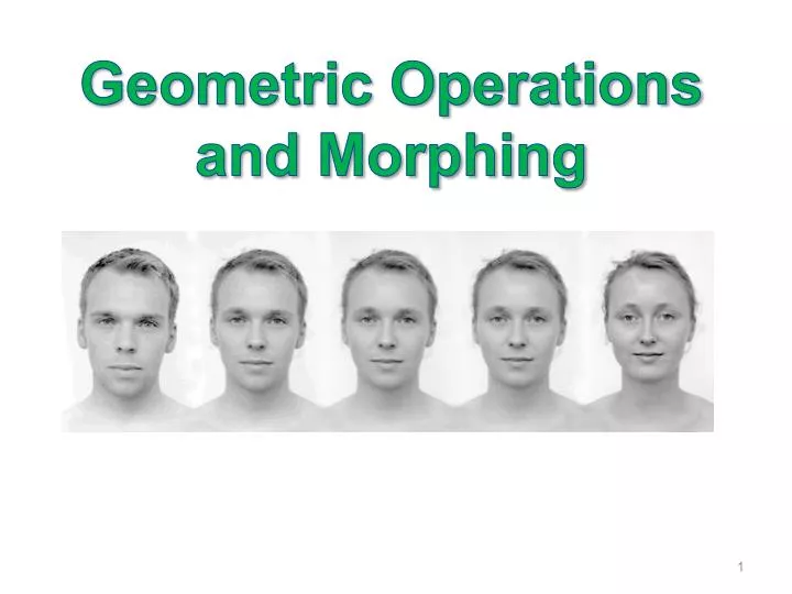
Geometric Operations and Morphing
Geometric Transformation • Operations depend on pixel’s Coordinates. • Context free. • Independent of pixel values. (x,y) (x’,y’) I(x,y) I’(x’,y’)
(x’,y’) • Example: Translation (x,y) I(x,y) I’(x’,y’)
Forward Mapping • Forward mapping: Target Source Forward Mapping
Forward vs. Inverse Mapping • Forward mapping: • Problems with forward mapping due to sampling: • Holes (some target pixels are not populated) • Overlaps (some target pixels assigned few colors) Target Source Forward mapping
Inverse mapping: • Each target pixel assigned a single color. • Color Interpolation is required. Source Target Inverse Mapping
Example: Scaling along X • Forward mapping: • Inverse mapping: Target Source (0,0) (0,0) Target Source
Interpolation • What happens when a mapping function calculates a fractional pixel address? • Interpolation: generates a new pixel by analyzing the surrounding pixels.
Interpolation • Good interpolation techniques attempt to find an optimal balance between three undesirable artifacts: edge halos, blurring and aliasing. x4 scaling N.N Bilinear Bicubic
Nearest Neighbor Interpolation • The assign value is taken from the pixel closest to the generated location: • Advantage: • Fast • Disadvantage: • Jagged results • Discontinues results
Nearest N. Interpolation Original Image
Original Image Nearest N. Interpolation
Bilinear Interpolation • The assigned value is an intermediate value between the four nearest pixels:
Linear Interpolation • Isolating v in the above equation: ve v vw xw x xe
Bilinear Interpolation • The assign value is a weighted sum of the four nearest pixels. • Each weight is proportional to the distance from each existing pixel.
N NW V NE • The bilinear interpolation is the best fit low-degree polynomial of the form: • The pixel’s boundaries are C0 continuous (continuous values across boundaries). S SE SW
Bilinear example s t s z=15 z=7 v t 0 1 z=2 z=3 0
Nearest N. Interpolation Bilinear Interpolation
Nearest N. Interpolation Bilinear Interpolation
Bicubic Interpolation • The assign value is a weighted sum of the 4x4 nearest pixels:
How can we find the right coefficients? • Denote the pixel values Vpq {p,q=0..3} • The unknown coefficients are aij {i,j=0..3} s • We have a linear system of 16 equations with 16 coefficients. • The pixel’s boundaries are C1 continuous (continuous derivatives across boundaries). t
N.N Bilinear Bicubic
Applying the Transformation T = …… % 2x2 transformation matrix [r,c] = size(img) % create array of destination x,y coordinates [X,Y]=meshgrid(1:c,1:r); % calculate source coordinates sourceCoor = inv(T) * [X(:) Y(:) ] ‘ ; % calculate nearest neighbor interpolation Xs = round(sourceCoor(1,:)); Ys = round(sourceCoor(2,:)); indx=find(Xs<1 | Xs>r); %out of range pixels Xs(indx)=1; Ys(indx)=1; indy=find(Ys<1 | Ys>c); %out of range pixels Xs(indy)=1; Ys(indy)=1; % calculate new image newImage = img((Xs-1).*r+Ys); newImage(indx)=0; newImage(indx)=0; newImage = reshape(newImage,r,c);
Types of linear 2D transformations • Rigid(Euclidean)transformation: • Translation + Rotation (distance preserving). • Similaritytransformation: • Translation + Rotation + Uniform Scale (angle preserving). • Affinetransformation: • Translation + Rotation + Scale + Shear (parallelism preserving). • Projective transformation • Cross-ratio preserving • All above transformations are groups where Rigid Similarity Affine Projective
Homogeneous Coordinates • Homogeneous Coordinates is a mapping from Rn to Rn+1: • Note: (tx,ty,t) all correspond to the same non-homogeneous point (x,y). E.g. (2,3,1)(6,9,3) (4,6,2). • Inverse mapping:
Some 2D Transformations • Translation : • Affine transformation: • Projective transformation:
Non Linear 2D Transformations • Non linear transformations do not necessarily preserve straight lines. • Methods: • Piecewise linear transformations • Non linear parametric mapping
Non linear mapping: • Example: non linear (radial) lens distortions:
Transformation Estimation • Let: x’=fx(x,y,px) ; y’=fy(x,y,py), where px and py are vector of parameters. • If the mappings are linear in px and py the parameters can be estimated using linear regression.
Example: Affine transformation • Alternative representation:
Given k points (P1,P2,..Pk) in 2D that have been transformed to (P'1,P'2,..,P'k) by affine transformation: • How many points uniquely define the affine (projective) transformation? • How can we find the affine transformation? • What if we have more points? • What can be done if points coordinates are inaccurate?
Image Warping and Morphing • Image rectification. • Key frame animation. • Image Synthesis • Facial expression • Viewing positions Image Metamorphosis.
Cross Dissolve (pixel operations) Source Image Destination Image t cross dissolve warp + dissolve
Warping + Cross Dissolve • Warp source image towards intermediate image. • Warp destination image towards intermediate image. • Cross-dissolve the two images by taking the weighted average at each pixel. source time Cross-dissolve destination warping images
warp Cross-dissolve Cross-dissolve warp
Image Metamorphosis • Let S,T be the source and the target images • Let G(p) be the transformation from S towards T, where G(0)=I the identity transformation • Let t[0,1] the time step to be synthesized Algorithm: • Warp S towards T: • Warp T toward S: • Cross dissolve:
t sourse S(t)=G(tp){S} I(t)=(1-t)S(t)+t(T(t)) target T(t)=G((1-t)p)-1{T}
Feature Based Morphing • Morph one shape into another shape • Use local features to define the geometric warping
Q Q’ P P’
Q Q’ P’ P
Q Q’ P’ P
Q Q’ P’ P
Q Q’ P’ P
Q Q’ P’ P
Q’ Q R R’ P P’ Source Image Dest Image One Segment Warping • [0,1] is the relative position along the segment (P’,Q’). • is the actual perpendicular distance to the segment. • (u’,v’) is the local coordinates of the segment (P’,Q’): • u’ is a unit vector parallel to Q’-P’ • v’ is the unit vector perpendicular to Q’-P’ v u u’ v’