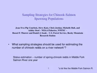
Sampling Strategies for Chinook-Salmon Spawning Populations

1. Sampling Strategies for Chinook-SalmonSpawning Populations • What sampling strategies should be used for estimating the number of chinook redds on a river network*? Status estimation – number of spring-chinook redds in Middle Fork Salmon River one year Jean-Yves Pip Courbois, Steve Katz, Chris Jordan, Michelle Rub, and Ashley Steel – NOAA Fisheries, NWFSC – Russel F. Thurow and Daniel J. Isaak – U.S. Forest Service, Rocky Mountain Research Station 1 *a lot like the Middle Fork Salmon R.

2. Chinook redds • At the conclusion of the annual spawning migration, adult female chinook prepare a spawning bed, a redd Disturbed gravels (light-colored area) indicate a Chinook redd Total number of redds is an indicator of population health, now and future 2

3. 0 10 20 40 Kilometers The Middle Fork Salmon River • National Wild and Scenic River in the Frank Church River of No Return Wilderness – roadless area • Drains about 7,330 km2 of central Idaho • Two level 4 HUCs and 126 level 6 HUCs • Home to 15 native fishes including 7 salmonid taxa • Spring chinook salmon – ESA listed • 655 km of chinook spawning reaches • Index reaches N 3

4. Number of redds – “the Truth” • Since 1995 we have counted the number of redds in the entire watershed via helicopter • Where necessary sampled by foot • This study uses six years of data: • These data will be considered the truth 4

5. Examples: Small and large runs 1995 2002 5

6. Objectives • Criteria • Design-based standard error of estimator • coverage probability (how many times 95% confidence interval actually contains the number of redds) • cost • Sampling and measurement unit: 200-meter reaches (N=3,274) • Keep things fair by sampling the same total length of stream, sampling fraction =.1 and .05 (n=327 and 164) • Although some standard errors can be calculated analytically the coverage needs to be addressed via simulation. 6

7. Methods • Use simulation by resampling the population over and over . . . 7

8. Costs & crew-trips • Each sampling unit in the MF is assigned to an access point • There are two types of access points: air fields and trailheads, same price • Cost for access sites = maximum distance from access site to sampling reaches in each “direction” along network • Total cost = sum of costs for 15 access sites 4 “directions” = 4 round trips required 8

9. Distances distances in 5km intervals. Maximum distance is 33 km. Many areas require over 20 km hike 9

10. The sampling strategies • Index – Sample the index reaches or SRS within index only. • Simple random sampling – • Cluster sampling – simple random sampling of 1 km. length units. • Systematic sampling – Sort tributaries in random order systematically sample along resulting line. • Stratify by Index – Sample independently within and outside the index regions. • Adaptive cluster sampling – Choose segments with a simple random sample. If sampled sites have redds sample adjacent segments. • Spatially balanced design – GRiTS, select segments as sampling units rather than points. 10

11. Index sampling • When the sample size is smaller than the overall size of the index region a simple random sample of the segments within the index is collected. • Two possibilities to estimate the number of redds from the index sample: • Assume there are no redds outside of the index – estimates will be too small (all) • Assume that the average number of redds per segment outside the index is the same inside and simply inflate the index estimator – estimates will be too large (rep) 11

12. Systematic sampling • Order the tributaries in random order along a line • Choose sampling interval, k, so that final sample size is approximately n • Select a random number, r, between 1 and k • Sample reaches r, r+k, r+2k, …, r+(n-1)k • Systematic sampling is cluster sampling where clusters are made up of units far apart in space and one cluster is sampled k r r+k r+2k r+3k r+4k 12

13. Stratify by Index • Stratify by index and oversample index reaches • Simple random sample in each stratum • Allocation: • Equal allocation: Usually does not perform well • Proportional allocation: Does not oversample index sites so will probably not have good precision • Optimal allocation: need to know the standard deviation 13

14. include neighbor Meets criteria and do not meet criteria 1 2 1 3 2 5 6 4 4 6 4 6 1 3 3 2 in original sample Adaptive cluster sampling • Original sample is simple random sample • If sampled site meets criteria also sample sites in neighborhood • Criteria: presence of redds • Neighborhood: segments directly upstream and downstream • Continue until sites do not meet criteria • Both legs of confluences • Two sample sizes: • ADAPT-EN – equate expected final sample size • ADAPT-N – equate original SRS sample size Meets criteria Final sample includes: 14

15. Results: Normalized standard error of estimators Run size 15

16. Standard error estimation for systematic strategy 16

17. Results: Empirical coverage probability • Empirical coverage probability Run size 17

18. Costs kilometers traveled 18

19. Relative precision per cost Precision per cost Units = 1/km traveled 10% sampling fraction 19 run size

20. Conclusions Precision • Medium to large runs: Systematic strategies (systematic and GRTS) • Standard error difficult to estimate for systematic strategy • Small runs: Stratified by index • Requires optimal allocation which is difficult to determine Cost and precision • Small runs – cheap strategies best, either index or SRS-1km • Medium runs – intermediately priced designs, stratify by index • Large runs – precise strategies best, either systematic strategies or stratified by index 20

21. Six years 1997 1998 21

22. Discussion • Adaptive cluster strategy is not as precise as other designs. • It is optimal for rare clustered populations • during small years the redds are not clustered enough • during large years they are not rare enough • only during the medium years does it compete with other designs • Many of the designs require extra information • Stratified • Adaptive • These results suggest more complex designs such as combining stratified with systematic or adaptive • Real vs. simulated data? 22

23. Acknowledgements • Tony Olsen (US-EPA), Damon Holzer, George Pess, (NOAA-Fisheries) • Funding for this research has been provided by NOAA-Fisheries Northwest Fisheries Sciences Center Cumulative Risk Initiative and partially by the US EPA cooperative agreement CR29096 to Oregon State University and its its subagreement E0101B-A to the University of Washington. • This research has not been formally reviewed by NOAA-Fisheries or the EPA. The views expressed in this document are solely those of the authors; NOAA-Fisheries and the EPA do not endorse any products or commercial services mentioned herein. Lucas Boone Courbois, born August 4, 2004 Seattle WA. 23

24. 24

25. Six years 1995 1996 25

26. Six years 2001 2002 26

27. Stratify by 6th field HUC 27

28. Points vs. Lines • Pick points -- points are picked along stream continuum and the measurement unit is constructed around the point • advantages: • different size measurement units are easily implemented • disadvantages: • difficulty with overlapping units • inadvertent variable probability design because of confluences and headwaters • Analysis may be complicated • Pick Segments – Universe is segmented before sampling and segments are picked from population of segments • advantages: • simple to implement • simple estimators • disadvantages: • Difficult frame construction before sampling • Cannot accommodate varying lengths of sampling unit 28

29. Methods • Sampling strategies include sampling design and estimator • Sampling and measurement unit: 3,274 200-meter segments • Measurement design assumes no measurement error Estimator for the total . . . sample design and confidence interval 29

30. Adaptive Cluster Sampling • Use the draw-by-draw probability estimator: • Let wi be the average number of redds in the network of which segment i belongs, then • with variance Thompson 1992 30

31. Access to MFSR • Roadless area • Airplane access possible 31

32. air vs. car access 32

33. Index sample • Not sure how to build estimates for total number of redds in Middle fork. • expand current estimator (assume same density outside of index) • use current estimate (assume 0 redds outside of index) 33

34. 34

35. Stratify by Index • Oversample index sites where most redds are located • Simple random sample in each stratum • Equal allocation: • Proportional allocation: 35

36. Stratify by index • Optimal allocation • Using 36

37. Stratify by index • Using 37

38. To do • stratified by 6th field HUC • Better estimators for Adaptive designs. • Cost function • including road/airplane travel • crew trips/day units 38