Introduction & Flood Hydrologic Analysis
Introduction & Flood Hydrologic Analysis. CE154 - Hydraulic Design Lectures 1-2. 1. Green Sheet. Course Objective - Introduce design concept and procedure for a few basic types of hydraulic structures that an engineer may encounter


Introduction & Flood Hydrologic Analysis
E N D
Presentation Transcript
Introduction & Flood Hydrologic Analysis CE154 - Hydraulic Design Lectures 1-2 CE154 1
Green Sheet • Course Objective - Introduce design concept and procedure for a few basic types of hydraulic structures that an engineer may encounter • Hydraulic structures:- Water supply and distribution systems including spillways, reservoirs, pipeline systems - Flood protection systems including culverts, storm drains, & natural rivers CE154 2
Green Sheet • Lecture Schedule • Homework assignments • Exams • Grading • Office hour • Communication – email address, web site • Emergency evacuation route • Grader selection CE154 3
Introduction • Hydraulic Design – Design of Hydraulic Structures • Elements of Design (class discussion)- design objective- design criteria - design data and assumptions- design procedure- design calculations- design drawings- design report CE154 4
Hydraulic Design example • Design a channel that can safely carry the storm runoff generated from a 1% flood from a residential development that is 20 square miles in drainage area. • Design objective: • Design criteria: • Design data and assumptions: • Design procedure: CE154 5
Flood Hydrology • Design flood Discharge (design flow)- peak flow rate governing the design of relevant hydraulic structures • Design flood Hydrograph- time-flow history of a design flood CE154 6
Sample Flood Hydrograph CE154
Hydrology • Rainfall – Runoff Process CE154 8
Hydrologic Parameters • Precipitationintensity & duration for design • Infiltration rate (watershed soil type and moisture condition) • Watershed surface cover – overland roughness • Watershed drainage network geometry • Watershed slope • Time of concentration CE154 9
Rainfall – Runoff Process • Gauged Watershed-flood frequency analysis to determine peak design flow rate-Gauge data to calibrate unit hydrograph and generate design flood hydrograph • Ungauged Watershed-Hydrologic Modeling (HEC-HMS or HEC-1)-Regional regression analysis-Synthetic unit hydrograph CE154 10
Flood Hydrology Studies • determine design rainfall duration and intensity- design rainfall ranges from probable maximum precipitation (PMP) on the high end to 100-year or 10-year return period rainfall event • develop design runoff hydrograph – includes peak flow rate and runoff volume to size reservoir and design spillway and other pertinent structures CE154 11
Our Topics • Determine probable maximum precipitation (PMP) -”Theoretically the greatest depth of precipitation for a given duration that is physically possible over a given storm area at a particular geographical location at a certain time of the year” (HMR55A) • Bureau of Reclamation’s S-graph & dimensionless unit hydrograph methods of developing synthetic unit hydrograph • Clark unit hydrograph method CE154 12
PMP • National Weather Service Hydrometeorological Reports (HMR)provide maximum 6, 12, 24, 48 and 72 hour PMP’s for areas of 10, 200, 1000, 5000 and 10,000 mi2.HMR 58 – Probable Maximum Precipitation for California – Calculation Procedures, NOAA, Oct. 1998 (supersedes HMR36, Note errata for pp. 22 & 27) • http://www.weather.gov/oh/hdsc/studies/pmp.html#HR58 CE154 13
Rainfall Losses • Surface retention, evaporation and storage (usually small compared to infiltration) • Infiltration- Ranges 0.05 0.5 in/hr approximately- L = Lmin + (Lo – Lmin)e-ktL = resulting infiltration rateLmin = minimum rate when saturatedLo = maximum or initial infiltration rate • Rainfall – losses = Rainfall Excess CE154 14
PMP Computation Example • Read pp. 43-48 of HMR 58 • 973 mi2 Auburn drainage above Folsom Lake • Step 1Outline drainage boundary and overlay the 10-mi2, 24-hour PMP map from Plate 2, HMR 58 • Step 2Determine to use all-season or seasonal PMP for design CE154 15
Plate 2 California – Northern General Storm PMP Index Map (in inches) CE154 16
PMP Computation Example CE154 17
PMP Computation Example • Step 3Calculate average PMP value (for 10 mi2 and 24-hr) over drainage area = 24.6 inches (using a planimeter or griddled paper overlay) • Step 4Depth-Duration Relationship- Auburn drainage is within the Sierra region. Use Table 2.1 to obtain ratios for durations from 1 to 72 hours CE154 18
PMP Computation Example CE154 19
PMP Computation Example CE154 20
PMP Computation Example • Multiply the average value for 10-mi2, 24-hour PMP of 24.6 inches by these ratios CE154 21
PMP Computation Example • Step 6Determine aerial reduction factors using the Auburn drainage area of 973 mi2 & Fig. 2.15 CE154 22
PMP Computation Example • Fig 2.15, HMR 58 CE154 23
PMP Computation Example CE154 24
PMP Computation Example • Step 7Apply aerial reduction by multiplying PMP’s from Step 5 by factors from Step 6 CE154 25
PMP Computation Example • Step 8Plot the depth-duration data on Fig. 2.19 CE154 26
PMP Computation Example • Extract cumulative depths from Fig. 2.19 CE154 27
PMP Computation Example • Compute incremental depths CE154 28
PMP Computation Example • Adjust temporal-distribution of these incremental rainfall based on historical data or by experiments. Keep the 4 highest increments in a series. A PMP isohyetal distribution may be CE154 29
PMP Computation - summary • Need Hydrometeorological Report HMR 58 for northern California • Define general storms up to 72 hours in duration and 10,000 mi2 in area and local storms up to 6 hours and 500 mi2 • Start with a total PMP depth for a general area and end with intensity-time distribution of rain for a specific watershed – this is the design rainfall CE154 30
How to turn PMP (design rainfall) into PMF (design runoff)? • Unit hydrograph – a rainfall-runoff relationship characteristic of the watershed - developed in 1930’s, easy to use, less data requirements, less costly- many methods, most often seen include Soil Conservation Service (SCS) method, Snyder, Clark, and Bureau of Reclamation dimensionless unit hydrograph and S-curve methods • hydrologic modeling – used widely since PC became popular, requiring data of topo contours, surface cover, infiltration ch., etc., HEC-HMS (HEC-1) CE154 31
Unit Hydrograph • Basic unit hydrograph theory A storm of a constant intensity over a duration (e.g, 1 hour), and of uniform distribution, produces 1 inch of excess that runs off the surface. The hydrograph that is recorded at the outlet of the watershed is a 1-hr unit hydrograph • Define several parameters to characterize the watershed response: e.g., lag time or time of concentration, time-discharge relationship, channel storage attenuation – synthetic unit hydrograph CE154 32
Unit Hydrograph Assumptions • Rainfall excess and losses may be lumped as basin-average values (lumped) • Ordinates of runoff is linearly proportional to rainfall excess values (linearity) • Rainfall-runoff relationship does not change with time (time invariance) CE154 33
Hydrograph Development CE154 34
Unit Hydrograph Approaches • Conceptual models of runoff – single-linear reservoir (S=kO), Nash (multiple linear reservoirs), Clark (consider effect of basin shape on travel time) • Empirical models – Snyder, Soil Conservation Service dimensionless method • Different methods use different parameters to define the unit hydrograph CE154 35
Unit Hydrograph Parameters • Time lag – time between center of mass of rainfall and center of mass of runoff, original definition by Horner & Flynt [1934], (SCS, Snyder). Different formulae were developed based on different watershed data (e.g., SCS & BuReC) • Time of concentration - time between end of rainfall excess and inflection point of receding runoff (Clark) • Time to peak – beginning of rise to peak (SCS) • Storage coefficient – R (Clark) • Temporal distribution of runoff (BuReC, SCS) CE154 36
Unit Hydrograph & parameters Rainfall excess = precipipation - loss Lag time Receding limb Q Time of concentration Point of inflection Rising limb Peak Time time CE154 37
Synthetic Unit Hydrograph • Uses Lag Time and a temporal distribution (dimensionless or S-graph) to develop the unit hydrograph CE154 38
Lag Time • Unit Hydrograph Lag Time (Tlag or Lg) per Bureau of Reclamation CE154 39
Lag Time • Lg = unit hydrograph lag time in hours • L = length of the longest watercourse from the point of concentration to the drainage boundary, in miles L Lca CE154 Point of concentration 40
Lag Time • Lca = length along the longest watercourse from the point of concentration to a point opposite the centroid of the drainage basin, in miles • S = average slope of the longest watercourse, in feet per mile • C, N = constant CE154 41
Lag Time • Based on empirical data, regardless of basin location • N = 0.33 • C = 26Kn where Kn is the average Manning’s roughness coefficient for the drainage network • Note: other methods such as Snyder and SCS define lag time slightly differently CE154 42
Lag Time • To allow estimate of lag time, the Bureau of Reclamation reconstituted 162 flood hydrographs from numerous natural basins west of Mississippi River to provide charts for lag time for 6 different regions of the US • Use Table 3-5 & Fig. 3-7 of DSD for lag time estimate for SF Bay Area CE154 43
Lag Time CE154 44
Lag Time • Example, Table 3-5 on p.42, DSD- San Francisquito Creek near Stanford University, drainage area 38.3 mi2, lag time 4.8 hours, Kn 0.110- Matadero Creek at Palo Alto, drainage area 7.2 mi2, lag time 3.7 hours, Kn 0.119 CE154 45
UH Temporal Distribution • Time vs. Discharge relationship • Bureau of Reclamation uses 2 methods to develop temporal distribution based on recorded hydrographs divided into 6 regions across the US:- dimensionless unit hydrograph method, &- S-graph technique • Tables 3-15 and 3-16 (Design of Small Dams) for the SF Bay Area CE154 46
Temporal Dist. – Table 3-16 CE154 47
Temp. Dist. - S-graph Method CE154 48
S-graph method - Example • Read pp. 37-52 of Design of Small Dams • drainage area = 250 mi2 • lag time = 12 hours • unit duration = 12/5 2 hours (SCS recommendation) • Ultimate discharge = drainage area in mi2 times 52802/3600/12 and divided by unit duration, in this case = 80662.5 cfs CE154 49
S-graph method - example CE154 50