abacus introduction
ABAQUS is a suite of finite element analysis modules. The heart of ABAQUS are the analysis modules, ABAQUS/Standard and ABAQUS/Explicit, which are complementary and integrated analysis tools.

abacus introduction
E N D
Presentation Transcript
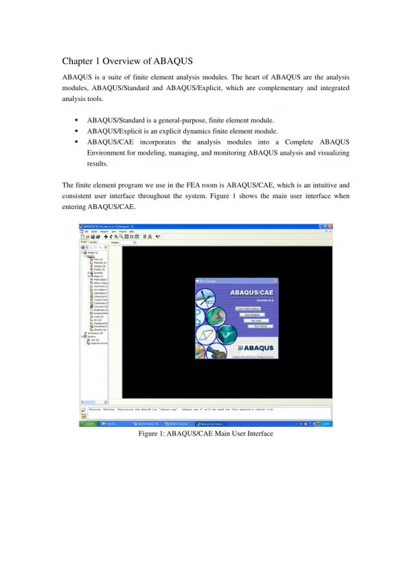
Chapter 1 Overview of ABAQUS ABAQUS is a suite of finite element analysis modules. The heart of ABAQUS are the analysis modules, ABAQUS/Standard and ABAQUS/Explicit, which are complementary and integrated analysis tools. ? ABAQUS/Standard is a general-purpose, finite element module. ? ABAQUS/Explicit is an explicit dynamics finite element module. ? ABAQUS/CAE incorporates the analysis modules into a Complete ABAQUS Environment for modeling, managing, and monitoring ABAQUS analysis and visualizing results. The finite element program we use in the FEA room is ABAQUS/CAE, which is an intuitive and consistent user interface throughout the system. Figure 1 shows the main user interface when entering ABAQUS/CAE. Figure 1: ABAQUS/CAE Main User Interface
Chapter 2 Launch and Exit ABAQUS 2.1 Steps to launch ABAQUS 1)Click Start - All programs – ABAQUS - ABAQUS 6.6.1 - ABAQUS Command in Windows System. An ABAQUS Command window appears in DOS environment (see figure 2 & 3). 2)Use general commands in DOS system to move to your directory on the hard disk. For example, if you have created a file in catalogue C:\Temp named ABAQUS WORK and you want all your ABAQUS results be saved in this file, you can type command CD C:\Temp\ABAQUS WORK. 3)Run command ABAQUS CAE to enter ABAQUS/CAE user interface as figure 1 shows.
Figure 2 & 3: Steps to Start ABAQUS/CAE 2.2 Starting a job in ABAQUS After entering main interface of ABAQUS/CAE, you have several paths to start a job. •Create Model Database allows you to begin a new analysis. •Open Database allows you to open a previously saved model or output database file. •Run Script allows you to run a file containing ABAQUS/CAE commands. •Start Tutorial allows you to begin an introductory tutorial from the online documentation 2.3 Exiting ABAQUS When you have done some work in the middle of an ABAQUS job and want to exit, you can save your finished work as a Model Database file (*.cae). • Click File – Save and input a file name (see Figure 4). Normally in this step the file filter is default to be Model Database (*.cae). • Click File – Exit to exit the main interface of ABAQUS/CAE. • Next time you run ABAQUS, you can just open the saved file and continue with the job.
Figure 4: Save a File in ABAQUS 2.4 ABAQUS Etiquette 1)It is a courtesy that you should be aware of the limited hard disk space of the computers in FEA room. Therefore, you should always free the disk space by doing the following things. You must delete all unnecessary files immediately after an ABAQUS analysis, such as *.stt, *.mdl, *.res, *.sta, *.msg. If you have already processed your results, you should delete *.fil, *.odb. Please always check your catalogue on the disk and keep deleting all unnecessary files as the system clogs up very quickly. Once the hard disk is full, nobody can do ABAQUS analysis. 2)Avoid running multiple jobs simultaneously as this uses up multiple licenses. Instead, run multiple jobs consecutively. It will take the save time. 3)Do not leave computers “locked” to other users for extended periods. ?
Chapter 3 Example: Compressive Response on a Steel Circular Hollow Tube In this example you will assess the response of a steel circular hollow tube subjected to a compressive load. The purpose of this example is to determine the response of the circular hollow section and see how it changes as the compressive load increases. We also aim to investigate the buckling load and yield load of the structure. 3.1 Create a model Use ABAQUS/CAE to create a three-dimensional model of the circular hollow tube section (CHS). The circular tube is constructed of 5 mm thick steel and is 400 mm diameter. The length of the tube could be 1200 mm for analysis. 3.1.1 Defining the model geometry 1)Start ABAQUS/CAE, and enter the Part module by clicking Part – Create. A dialog box of Create Part appears as Figure 5 shows. Figure 5: Create Part 2)In the dialog box, create a 3D, deformable part with an extruded shell base feature to represent the CHS (See Figure 5). Use an approximate part size of 1000, and name the part CHS. 3)Click the button Create Circle: Center and Perimeter tool to sketch a circle with 400 mm diameter.
4)Pick center point at (0, 0) and perimeter point at (0,200) or (200, 0) to define the circle geometry. The section sketch is shown in Figure 6. 5)When finish sketching the section, end the Create Circle: Center and Perimeter tool by clicking that button once again, and there appears a hint ‘Sketch the section for the shell extrusion’. Click Done. Set the depth 1200 mm. After that, the sketch is extruded to a depth of 1200 mm and a circular tube is therefore created. The final part is shown in Figure 7. Figure 6: Section Sketch
Figure 7: The Final Part of CHS 3.1.2 Defining the material properties In the Module selection, select and click Property to define the material and section properties. Assume that the CHS is made of steel, with a Young’s modulus of 210 GPa, a Poisson’s ratio of 0.3. At this stage we do not know whether there will be any plastic deformation, but we know the value of the yield stress and the details of the post-yield behavior for this steel. We will include this information in the material definition. The plasticity data and stress-strain curve are shown in Figure 8. Material properties Elastic properties: = 200 10 Pa, × ν = 9 0.3 E Plastic properties: True Stress (MPa) True Strain 400 400 460 500 0.00 0.03 0.05 0.08 Figure 8: Plasticity Data and Stress-strain Curve
Yield Stress (MPa) 400 400 460 500 Plastic Strain 0.00 0.03 0.05 0.08 Figure 9: The Yield Stress and Plastic Strain Data Input in ABAQUS 3.1.2.1 Create material To define an elastic-plastic material: 1)Click the button Create Material. The Edit Material dialog box turns up. Name the material Steel. 2)In the Edit Material dialog box, select Mechanical – Elasticity – Elastic to define the elastic material properties. Enter 200E9 Pa as the value for Young’s modulus and 0.3 as the value for Poisson’s ratio. 3)Select Mechanical – Plasticity – Plastic to define the plastic material properties. Enter the yield stress and plastic strain data shown in Figure 9. You can click Material Manager to check if the properties are correctly entered as Figure 10 shows. Figure 10: Material Manager You should note that ABAQUS is numerical and hence it does not have default units. You need therefore to be consistent in using units when defining geometry, loads and material properties. In
this example, we used mm as the unit of dimension in defining the geometry and presume the unit of load to be N, then the unit of stress and Young’s modulus should be MPa. 3.1.2.2 Creating and assigning section properties To create homogeneous shell section properties and refer to the steel material definition and shell thickness: 1)Click Create Section. The Create Section dialog box appears. Name the shell section property SteelSection, select Shell Homogeneous and continue. 2)In the Edit Section dialog box, select Steel as the material, and specify 5 mm as the value for the Shell thickness. Then press OK. You can click Section Manager to check or modify the section properties in the dialog box as Figure 11 shows. Figure 11: Section Manager To assign the SteelSection definition to the regions of the steel circular tube: 1)Click Assign Section. 2)Click the entire circular tube as the regions to be assigned a section, and press DONE. 3)Press Ok in the Edit Section Assignment dialog box. You can click Section Assignment Manager to check or modify the section assignment in the dialog box as Figure 12 shows.
Figure 12: Section Assignment Manager 3.1.3 Creating an assembly 1)Enter the Assembly module, and click Instance Part. 2)As shown in Figure 13, select CHS as the part, and use the default coordinate system. Figure 13: Creating Assembly
It is simple to create an assembly for an integrated structure such as this example. However, some models may be complicated if they are composed of several small parts which have different material properties. You should define the material properties for each part in the previous steps and assemble them in this step. 3.1.4 Creating the mesh 1)Enter the Mesh module to seed the part instance. 2)Select Seed – Edge By Number and specify that 60 elements be created along the perimeter of the circular section. To do so, click the perimeter as the region to be assigned local seeds and press DONE. Then enter 60 as the number of elements along the edge. 3)Select Mesh – Controls, and use the default element shape and press OK. 4)Select Mesh – Element Type, and use the default quadrilateral shell elements (S4R) as the element type to be applied in this case. 5)Select Mesh – Part, and press OK to mesh the part. Figure 14: Meshed CHS The resulting mesh is shown in Figure 14. This relatively coarse mesh provides moderate accuracy while keeping the solution time to minimum. You can create finer mesh to get more accurate solution which however takes longer when running the job. You should carefully consider what type of element should be used before meshing a model. Different element types may make significant difference. Check more details in relevant ABAQUS manuals.
3.1.5 Defining steps 1)Enter the Step module. 2)Select Step – Create, and name a new step as Buckle after the initial one. As for the procedure type, select Linear perturbation – Buckle. 3)In the Edit Step dialog box, specify the following step description: Buckle. Enter 5 as the number of eigenvalues requested. Enter 10 as the vectors used per iteration, and enter 1000 as the maximum number of iterations. Press OK. You can click Step Manager to check or modify the steps in the dialog box as Figure 15 shows. Figure 15: Step Management 3.1.6 Prescribing boundary conditions and loads 1)Enter the Load module to define the boundary conditions used in this analysis. 2)Select Tool – Set – Create, and create a set named Fixed, select the perimeter edge of one end of the CHS as the geometry of the set, and press DONE. Similarly, create another set named Moving by selecting the other end of the CHS. Then, create a set named Displacement, and click one node point of the moving end as the geometry. Enter Set Manager to check the three sets, as shown in Figure 16.
Figure 16: Set Manager 3)Select BC – Create, and create a boundary condition in the Initial step named Fixed Edge. Select Mechanical – Displacement/Rotation to be the type of step. Apply the boundary condition to the set of Fixed by clicking Set in the right corner and selecting Fixed. In the Edit Boundary Condition dialog box, tick U1, U2, U3, UR1, UR2, UR3 to fully constrain the set (U1 = U2 = U3 = UR1 = UR2 = UR3 = 0). Press OK. See Figure 17.
Figure 17: Create Fixed Edge 4)Select BC – Create, and create another boundary condition in the Buckle step named Moving edge. Select Mechanical – Displacement/Rotation to be the type of step. Apply the boundary condition to the set of Moving by clicking Set in the right corner and selecting Moving. In the Edit Boundary Condition dialog box, keep the default settings and tick U1, U2, U3, UR1, UR2, UR3 and specify U3 as -2 (U1 = U2 = UR1 = UR2 = UR3 = 0, U3 = -2). Press OK. See Figure 18.
Figure 18: Create Moving Edge The boundary conditions applied is shown in Figure 19. Figure 19: Boundary Conditions
3.2 Analysis - Estimating buckling stress In this example, eigenvalue buckling analysis was generally used to estimate the critical bucking loads of the CHS. An incremental loading pattern was defined in *BUCKLE step (Fixed edge: U1 = U2 = U3 = UR1 = UR2 = UR3 = 0; Moving edge: U1 = U2 = UR1 = UR2 = UR3 = 0, U3 = -2). A general eigenvalue buckling analysis can provide useful estimates of collapse mode shapes and calculate the buckling stress as well. 3.2.1 Defining and submitting a job 1)Enter the Job module, create a job named Buckle. Specify the following job description: Buckle. 2)Save your model in a model database file, and submit the job for analysis. Monitor the solution progress; correct any modeling errors that are detected, and investigate the cause of any warning messages. 3.2.2 Postprocessing 3.2.2.1 Visualization of results Enter the Visualization module, and open the .odb file created by this job (Buckle.odb). You can view the following shapes or plots by clicking corresponding tool buttons: ? Undeformed shape; ? Deformed shape; ? Animation of results; ? Contour plots; ? Eigenvalue. Figure 20 shows the contour plot of spatial displacement at nodes.
Figure 20: Contour Plot of Spatial Displacement at Nodes in Eigenvalue Analysis 3.2.2.2 Calculation of buckling stress The equation for calculation of buckling stress can be written as follows: Δ l σ = ⋅ ε = λ ⋅ ⋅ E E cr l where E is the material Young’s modulus, λ is the eigenvalue obtained from the results of FEA, l Δ is the initial displacement at the movable end input in the boundary conditions (U3 = -2) in ABAQUS, l is the length of the column. The results show that λ = 9.0471. Apply 200 10 E = equation, and therefore the buckling stress can be calculated. As a result, 3.3 Analysis - Compressive response on CHS The objective of this analysis is to study the deformation of the CHS and the stress-strain response in various parts of the structure when it is subjected to a compressive load. 3.3.1 Modify model 1)Enter the Step module. 2)Replace step Buckle with Geneal – Static, Riks. 3)In the Edit Step dialog box, specify the following step description: Analysis. Turn Nlgeom On. In the Incrementation box, specify Arc length increment as followings: Initial = 0.01, Minimum = 1e-20, Maximum = 1. Press OK. × Δ = = 9 , 2 , 1200 3.02 Pa L mm L σ mm GPa in the . = cr
3.3.2 Defining and submitting a job 1)Enter the Job module, create a job named Analysis. Specify the following job description: Analysis. 2)Save your model in a model database file, and submit the job for analysis. 3.3.3 Running and monitoring job process The objective of this analysis is to observe the stress-strain response of the CHS under compression. In the process of the job, you can monitor the solution progress by clicking Results in the dialog box of Job Manager and see the changing of stress allocation during the whole analysis. For this example, once the maximum stress of CHS reaches ultimate, which means some part of the CHS has yielded, you can terminate the analysis by clicking Kill in the dialog box. The job will therefore be aborted, however, all the response before the termination can be observed. 3.3.4 Postprocessing 3.3.4.1 Visualization of results Enter the Visualization module, and open the .odb file created by this job (Analysis.odb). You can view the following shapes or plots by clicking corresponding tool buttons: ? Undeformed shape; ? Deformed shape; ? Animation of results; ? Contour plots. Figure 21 shows the deformed shape of CHS in the analysis. Figure 21: Deformed Shape of CHS
3.3.4.2 Data processing This section mainly introduces how to obtain a data plot of load-displacement in the movable end of CHS. The principle is to collect the data of reaction force in the fixed end of CHS and the data of the displacement of the movable end. Both of them are in the z-coordinate direction. 1)Select Tool – XY Data – Manager – Create – OBD field output, there appears a dialog box. 2)Collect the data of reaction forces. In the catalogue of Variables, select Position as Unique Nodal. Then select RF3 (Reaction force in the direction of z-coordinate). In catalogue of Elements/Nodes, click Node sets – Fixed. Then press Save – OK. 3)Collect the data of displacement. In the catalogue of Variables, select Position as Unique Nodal. Then select U3 (Displacement in the direction of z-coordinate). In catalogue of Elements/Nodes, click Node sets – Displacement. Click Save – OK. Close the dialog box. 4)Select Tool – XY Data – Manager – Create – Operate on XY data, there appears a dialog box. 5)Row down the operation functions column on the right side, and click sum((A, A,…)). Multi-select all the RF3 data and click Add to Expression. Save as RF3. 6)Click Clear Expression. Row down the operation column to click combine (X, X). Select U3 to Add to Expression and then RF3 (which was saved in the above procedure) to add to expression. Give a negative sign to U3, as the displacement is in the negative direction of z-coordinate while we hope the see the plot which displacement is positive. Save as plot. 7)Click Plot Expression, the Load-Displacement diagram is shown as Figure 22. Figure 22: Plot of Load-displacement Response
Alternatively, you can do the following to save all the data of the plot as an Ms-Excel file. 1)Click Report – XY. 2)In the catalogue of XY Data, click plot. 3)In the catalogue of Setup, name a file xxx.xls and save in the hard drive. 4)Click OK. Note: You must save it as an Excel file, otherwise it cannot be read. Check this file and you would find all the detailed data are included in. You can also make diagrams using these data. See Figure 23. Figure 23: X-Y Data Saved as a MS-Excel File For further guidance, look up ABAQUS 6.4 online documentation - http://129.78.142.16:2080/v6.4/