SMILE! You’re on Traffic Light Camera: Applying Stated Choice Modeling in Transportation
SMILE! You’re on Traffic Light Camera: Applying Stated Choice Modeling in Transportation. W. Douglass Shaw (presenter) Dept. of Agricultural Economics and Recreation, Parks and Tourism Sciences April 14, 2008. Acknowledgments.


SMILE! You’re on Traffic Light Camera: Applying Stated Choice Modeling in Transportation
E N D
Presentation Transcript
SMILE! You’re on Traffic Light Camera: Applying Stated Choice Modelingin Transportation W. Douglass Shaw (presenter) Dept. of Agricultural Economics and Recreation, Parks and Tourism Sciences April 14, 2008
Acknowledgments • The graduate students in this semester’s Ag. Econ. 695 (Frontiers in Natural Resource and Environmental Economics) and RPTS 616 (Economics of Tourism and Recreation) • Especially Lindsey Higgins (Ag. Econ.), Liam Carr (Geography) • Conversations on CM with Bill Breffle (and 2 of his slides), Barbara Kanninen, Edward Morey, Mary Riddel
My Main Contributionto Economics? • Probably… • We (Pete Feather and I) showed that people can have an opportunity cost of their time that exceeds their wage rate (see Economic Inquiry 2000; J. of Environmental Economics and Management 1999) • Are there any applications to transportation of that…?
Links to Transportation? • Somebody apparently thought so • Peter is now the Chief of the Fuel Economy Division at the United States Department of Transportation… • He is an “environmental and natural resource” economist
Outline / Preview • Hope: I could present some statistical results from the graduate seminar class project on “choice modeling” • Not quite ready, but I’ll show you what we have so far. • So, this talk is an overview of stated choice modeling method and how it can be applied to some transportation issues. • What are experimental/economic choice models and how can these be used to model transportation-related preferences and behaviors?
Audience Knowledge? • How many here today know about stated choice models as a tool that can be used to evaluate transportation-related preferences? • Some big “transportation” names of people who have done this kind of modeling include: C. Bhat, Dan McFadden, Moshe Ben Akiva, David Hensher, S. Lerman, Jordan Louviere, Charles Manski, Kenneth Train • Not sure any of these people are exclusively “transportation” researchers per se. • Lots of SCM papers published recently in the journals Transportation, Transportation Research, Transport Policy, Journal of Transportation Economics and Policy, etc.
A Little Technical Stuff • Choice modeling is similar to “Conjoint” analysis • Stated Preferences/choices/rankings can be used (so can data from “actual” or “real” choices) • Most use “discrete” choice analysis (econometrics) • Designs vary from: • Paired Designs (Choose A or Choose B) • Multiple Choice Designs (Choose one from A,B,C) • Rank these routes (more often done in conjoint)
Discrete Choice Econometrics • As there are typically few choices, the error terms are not continuously/normally distributed; rather, they relate to discrete distributes • The old standard is to use the extreme value distribution leading to the logit or multinomial logit • The new standard is to use the “mixed” or random parameters logit, or perhaps, a panel (fixed or random effects) logit model
Experiments? • Laboratory experiments are designed to control for every aspect that influences the outcome • Choice experiments seek the same level of control • Unlike using revealed preference data (e.g. data on your actual trips) the researcher here constructs every aspect of a choice alternative in a stated choice model (SCM) • Choices can be made in a computer laboratory setting
Another Advantage of SCMs • Suppose you want to “market” a new product or idea? • The idea is a plan, as in a planned new transportation route or alternative • Define the attributes of the new route and develop an SCM • In Transportation: New airline, bus route service; new airplane configuration (more leg room); the new Texas highway; toll roads; new HOV lanes; congestion taxes, new parking facilities; new sidewalks; new traffic lights; remove traffic lights; rotaries (new Beaver Creek, Colorado), etc, etc…
Essentials of Experimental Design • The Alternatives • The Attributes of the alternatives • The Levels of the attributes • How are these designed so as to elicit the most information possible without increasing the complexity such that individuals cannot perform the experiment?
A Little More Jargon • A “profile” is a single alternative that is described by the levels of each attribute • A “choice set” is a set of alternatives (two or more) presented to the individual, e.g. A versus B, or A versus B versus C, where each letter is a profile and the combination is a choice set • Researcher has to first figure out how many profiles are needed, then how many choice sets
The Alternatives • Does a person look at two at once? • Or three? • Or four (or more)?
Attributes Characterize Alternatives (the Choices) • e.g.: What are the attributes of a commuting alternative that matter to people? • Cost (money and time) • Comfort • Discretionary power (flexibility in choosing schedule) • Reliability
Levels Determine Definition of the Alternative • What are the money prices? • Range from “free” to calculations based on parking, toll roads, gasoline prices, mpg of the vehicle • e.g. Local prices per trip are: {$0, $1, $2.50, $5.00, $8.00} • What are the times? • Range from few minutes to hours • e.g. Local commuting times per trip (including all parts of the trip): {5 min., 10 min, 20 min, 30 min, 1 hour) • Comfort (low, medium, high); Reliability (very unreliable, sometimes unreliable, always reliable)
How Many Possibilities? Design • L levels, K attributes LK = possible “profiles” • Full factorial design considers all possible profiles • Possible? • Example of Commuting Attributes (# of Levels) • Price (five), Time (five), Comfort (three), Flexibility (three), Reliability (three) • 52 X 33 = 25 X 27 = 675
Quickly Exploding • I didn’t probably get all the attributes or levels covered. If more… • Can you “cover” 1,000 profiles? • No • So, what to do? That’s the art of design • Fractional factorial design
Key Design Components (Huber and Zwerina) • Level Balance: Each level of each attribute should appear with equal frequency • Orthogonality: mathematical independence to allow identification of parameters: • Satisfied when joint occurrence of any 2 levels of different attributes appear in profiles with frequencies = the product of their marginal frequencies • Simply: attributes are purposefully uncorrelated (makes it easier to identify variable X’s influence)
Key Design Components (cont.) • Minimal Overlap: the probability that an attribute level repeats itself in a choices set is minimized • Utility Balance: Balance the utility received: Avoid dominance of choices, the probability of choosing each alternative should be fairly even
Quantitative measures of efficiency:D-optimal efficiency The D-optimal criterion seeks to maximize the determinant of the Fisher information matrix Max: D = 100{1/N|(X’X)-1|1/A N = number of observations; A is number of attributes*levels in design; X’X is the information matrix • Uninformed prior – all parameters equal zero • A priori information based on pretest or other data • Bayesian information hierarchically added
Conclusions about D-criterion • D-efficiency preferred when specification and design are both correct • D-efficiency with Bayesian info preferred when specification is incorrect but design is correct • “Shifting” preferred to D-efficiency when the specification is correct but the design is not • Most common • If design is correct, do not need a design-creating process! • Also known as cycling
Alternatives using D-criterion • Fractional design drawn multiple times, with D-criterion compared for each draw • “Frequentist” model averaging: design evaluated over a distribution of parameter values and final design is a weighted average (uses partial info)
Class on Choice Modeling: An Example Project • Agricultural Economics 695 (PhD seminar) • Recreation, Parks, and Tourism Sciences (616 – PhD course) • Assignment: Design a choice modeling experiment that has something to do with transportation issue in Bryan/College Station
Students’ Decision • Identify the impact of CARES (Camera Advancing Red Light Enforcement Safety) on driver behavior, road and traffic safety, and pedestrian safety • Installation of red light cameras, coupled with $75 citation for violations • Expansion of the program planned • No funding, so using convenience sample and internet survey
Student News Item • The Battalion (April 9, 2008) – Nathan Ball • 3,318 citations as of April 1st, generating $248,859 (four existing cameras) • Of existing fines, 659 mailed to College Station residents
Design • Four attributes: # of cameras; the location of the intersections for installation; the cost of the fine; the posted speed limit (mph) • Student in the class used SAS Optex procedure • 16 “profiles” (see next slide)
Next Step • Suppose we want to create a pair of profiles to evaluate and ask the person to choose profile 1 versus profile 2. • Does it matter which profiles are paired? • Yes • How do we match them? • Answer is complicated and there are many schemes that try to achieve an efficient design based on the four goals above.
Example • Do we want choice A to be profile 1 and choice B to be profile 2? From the original profiles, we’d get: • Choose between A (4 cameras, citation fine is $50, cameras at current locations, speed is reduced) and B (4 cameras, citation fine is $74, cameras at current locations, speed is reduced) • Only thing that varies between A and B is the citation/fine amount
See Their Survey • http://geography.tamu.edu/cares_survey/ • Aside on Internet surveys • See Knowledge Networks Inc. (webcast of presentation on survey bias, April 24th) • Wave of the future?
For each section read any instructions and each question carefully before answering. Please do not leave any answers blank. An answer of N/A is provided for questions you’d choose to not answer. Thank you again for taking the time to complete this survey. Current Residency: College Station Bryan Neither Prior to taking this survey, of the four intersections with red light cameras, how many can you confidently name or locate? 0 1 2 3 4 The map shows the location of red light cameras in the College Station CARES Program. The cameras carry a $75 citation at intersections of roads with a 40 mph speed limit. For the purposes of this survey, these four cameras will remain in use. For each question, you will be given two alternatives for changing the CARES Program. The alternatives may change the cost of the citation, the speed limit, number of additional cameras, and placing additional cameras at intersections with high pedestrian traffic, high road volume, or a mix of intersections throughout College Station. Based on the information and your own personal knowledge, select the alternative you prefer.
Initial Thought • Not everyone thinks cameras are “good” in safety – may be revenue for town • They might focus on speed limit • Had hoped to have at least some more preliminary statistical results on this one • In the “field” giving surveys • No complete data set yet
Thoughts on CM Applications to Some Other Texas Transportation Issues • Hurricane evacuation behavior and risk perceptions • What is the risk that a hurricane will hit? • Given this, will you evacuate? Perhaps add, how long before you do? (could add the risks of getting caught in a traffic jam, which are function of when you leave) • “New” routes through rural and other areas? • Biking v. Driving as the cost of gasoline increases…
Application(UTCM project w/ Mark Burris) • Managed Lanes (less congestion, but pay a toll for this) • Katy Freeway • Will people use it/the ML’s? • What will they willing to pay in tolls? • What is the value of ML’s? Managed Lanes (ML) offer travelers the option of congestion free travel in corridors where the general purpose lanes (GPL) are congested. To ensure the MLs do not become congested (and often to help pay for the construction of the lanes) travelers have to pay a toll to use the MLs. This toll varies by time of day or by congestion level, increasing as demand for the lane increases. Thus travelers have to make a decision, often at the spur of the moment, on use.
If Time Allows: Another Example • NSF Hurricane Project • Small Exploratory Grants Research (SGER) Program • Look at victims from Katrina/Rita who had relocated here or in Houston • Examine their location preferences for moving back or elsewhere using a choice model • Also look at their subjective perceptions of risk (just after the hurricanes in 2005, and over one year later)
Two Rounds • Round I – mostly from B/CS – living here “temporarily” • Round II – from B/CS and from Houston (we lost many from Round I – no one knows where they went) • Compare risks and behaviors in model of all subjects
Empirical Approach • Tried two panel logit specifications (η is normally distributed individual-specific component, T is # of observations per person i). Log likelihood (random effects):
Marginal WTP (One time) • High Risk to None • Round I $10,100 • Round II $4,800 • High Risk to Medium Risk • Round I $6,550 • Round II $3,456
Results from Hurricane Study(in words) • Key: • Risks matter: higher risks, less likely to choose that location • Risks still matter to both groups, but matter less a year later • People do NOT want to all go back to New Orleans • Net income (income less housing costs) increases chance of picking a location