Congestion and crowding Games
Congestion and crowding Games. Pasquale Ambrosio* Vincenzo Bonifaci + Carmine Ventre * *University of Salerno + University “La Sapienza” Roma. What is a game?. Classical example: BoS game Players Strategies: S 1 = S 2 = {Bach, Stravinsky}

Congestion and crowding Games
E N D
Presentation Transcript
Congestion and crowding Games Pasquale Ambrosio* Vincenzo Bonifaci+ Carmine Ventre* *University of Salerno +University “La Sapienza” Roma
What is a game? • Classical example: BoS game • Players • Strategies: S1 = S2 = {Bach, Stravinsky} • Payoff functions: u1(B,B) = 2, u2(B,S) = 0, … • Equilibria: i.e. (B,B) and (S,S) are Nash equilibria Bach Stravinsky A strategy s (e.g. (B,B)) is a Nash equilibrium iff for all players i it holds: ui(s-i,s) >= ui(s-i,s’) for each s’ in Si Bach player 1 Stravinsky player 2
(General) Congestion Games • resources • roads 1,2,3,4 • players • driver A, driver B • strategies: which roads I use for reach my destination? • A wants to go in Salerno • e.g. SA={{1,2},{3,4}} • B wants to go in Napoli • e.g. SB={{1,4},{2,3}} • what about the payoffs? A B Roma Milano road 1 road 4 road 2 road 3 Napoli Salerno
Payoffs in (G)CG: an example A SIRF (Small Index Road First) B • A choose path 1,2 • B choose path 1,4 • uA = - (c1(2) + c2(1)) = - 4 • uB = - (c1(2) + c4(1)) = - 5 Roma Milano road 1 road 4 road 2 road 3 Napoli Salerno B Costs for the roads {1,4} {2,3} c1(1)=2 c1(2)= 3 c2(1)=1 c2(2)= 4 c3(1)=4 c3(2)= 6 c4(1)=2 c4(2)= 5 {1,2} A {3,4}
Payoffs in (G)CG • The payoff of i depends by congestion of the selected resources • ui is the opposite of the total congestion cost paid by i (Ci) • For each resource there is a congestion cost (or delay) ck • ck is function of nk(s) (the number of players that in the state s choose the resource k) • Therefore the payoff of i in the state s is:
Congestion games: various models • Symmetric CG • Si are all the same and payoffs are identical symmetric function of n-1 variables • Single-choice CG • Each player can choose only one resource (anyone in the resources set E) • Unification of concepts of strategies and resources • Subjective CG • Each player has a different experience of the congestion • As consequence every player has a specific payoff
Congestion games: various models (2) • Network CG • Each player has a starting and terminal node and the strategies are the paths in the network • Crowding game • Single-choice subjective CG with payoff non-increasing in nk(s) • Weighted crowding game • Each player has a different weight upon the congestion
Every game has at least one mixed Nash equilibrium A game with pure equilibria is “better” than another one with just mixed equilibria GCG and pure Nash equilibria Thm (Rosenthal, 1973) Every (general) CG possesses at least one pure Nash equilibrium.
Rosenthal’s result • The class of GCG is “nice” • We know that there is a class of game for which it is possible to find a pure equilibrium (algorithm?) • Introduce this (potential) function:
Potential functions • A potential function can trace the “global payoff” of the system along the Nash dynamics • Several kind of potential functions: • Ordinal potential function • Weighted potential function • (Exact) potential function • Generalized ordinal potential function
Ordinal potential function • A function P (from S to R) is an OPF for a game G if for every player i • ui(s-i, x) - ui(s-i, z) > 0 iff P(s-i, x) - P(s-i, z) > 0 • for every x, z in Si and for every s-i in S-i BoS = P1 = u1(B,B) – u1(S,B) > 0 implies that P1(B,B) – P1(S,B) > 0 u1(B,S) – u1(S,S) < 0 implies that P1(B,S) – P1(S,S) < 0 P1(B,B) – P1(S,B) > 0 implies that u1(B,B) – u1(S,B) > 0 and that u2(B,B) – u2(S,B) > 0 P1 is an ordinal potential function for BoS game
A B (3,1) (4,0) 11 9 A P3 = G’ = (2,4) (1,0) 8 0 B u1(A,A) – u1(B,A) = 3 - 2 = 1/3 (P3(A,A) – P3(B,A)) P3 is a (1/3,1/2)-potential function for the game G’ u1(A,B) – u1(B,B) = 4 - 1 = 1/3 (P3(A,B) – P3(B,B)) u2(B,A) – u2(B,B) = 4 - 0 = 1/2 (P3(B,A) – P3(B,B)) u2(A,A) – u2(A,B) = 1 - 0 = 1/2 (P3(A,A) – P3(A,B)) Weighted potential function • A function P (from S to R) is a w-PF for a game G if for every player i • ui(s-i, x) - ui(s-i, z) = wi (P(s-i, x) - P(s-i, z)) • for every x, z in Si and for every s-i in S-i C D C P2 = PD = D u1(C,C) – u1(D,C) = 1 = 2 (P2(C,C) – P2(D,C)) u1(C,D) – u1(D,D) = 3 = 2 (P2(C,D) – P2(D,D)) P2 is a (2,2)-potential function for PD game u2(D,C) – u2(D,D) = 3 = 2 (P2(D,C) – P2(D,D)) u2(C,C) – u2(C,D) = 1 = 2 (P2(C,C) – P2(C,D))
(Exact) potential function A function P (from S to R) is an (exact) PF for a game G if it is a w-potential function for G with wi = 1 for every i C D C P4 = PD = D u1(C,C) – u1(D,C) = P4(C,C) – P4(D,C) u1(C,D) – u1(D,D) = P4(C,D) – P4(D,D) P4 is a potential function for PD game u2(D,C) – u2(D,D) = P4(D,C) – P4(D,D) u2(C,C) – u2(C,D) = P4(C,C) – P4(C,D)
Generalized ordinal potential function A function P (from S to R) is an GOPF for a game G if for every player i ui(s-i, x) - ui(s-i, z) > 0 implies P(s-i, x) - P(s-i, z) > 0 for every x, z in Si and for every s-i in S-i A B A G’’ = P5 = B P5 is a generalized ordinal potential function for the game G’’ P5 is not an ordinal potential function for the game G’’ P5(A,B) – P5(A,A) > 0 implies that u1(A,B) – u1(A,A) > 0 but not that u2(A,B) – u2(A,A) > 0
Potential games • A game that admits an OPF is called an ordinal potential game • A game that admits a weighted PF is called a weighted potential game • A game that admits a PF is called a potential game • Using the potential functions properties we obtain several interesting results • E.g., in such games find an equilibrium is equivalent to maximize the potential
Equilibria in Potential Games Thm (MS96) Let G be an ordinal potential game (P is an OPF). A strategy profile s in S is a pure equilibrium point for G iff for every player i it holds P(s) >= P(s-i, x) for every x in Si Therefore, if P has maximal value in S, then G has a pure Nash equilibrium. Corollary Every finite OP game has a pure Nash equilibrium.
An example Nash equilibrium P4 maximal value C D C P4 = PD = D Thm (MS96) C D C PD(P4) = D
FIP: an important property • A path in S is a sequence of states s.t. between every consecutive pair of states there is only one deviator • A path is an improvement path w.r.t. G if each deviator has a sharp advantage moving ui(sk) > ui(sk-1) • G has the FIP if every improvement path is finite • Clearly if G has the FIP then G has at least a pure equilibrium • Every improvement path terminates in an equilibrium point
FIP: an important property (2) Lemma Every finite OP game has the FIP. The converse is true? “No” • G’’ has the FIP ((B,A) is an equilibrium) • any OPF must satisfies the following impossible relations: • P(A,A) < P(B,A) < P(B,B) < P(A,B) = P(A,A) A B A G’’ = B Lemma Let G be a finite game. Then, G has the FIP iff G has a generalized ordinal potential function.
Congestion vs Potential Games • Rosenthal states that Congestion games always admit pure Nash equilibria • MS96’s work shows that potential games always admit pure Nash equilibria • What is the relation? Thm Every congestion game is a potential game. Thm Every finite potential game is isomorphic to a congestion game.