On Difference Variances as Residual Error Measures in Geolocation
250 likes | 611 Vues
On Difference Variances as Residual Error Measures in Geolocation Victor S. Reinhardt Raytheon Space and Airborne Systems El Segundo, CA, USA ION National Technical Meeting January 28-30, 2008 San Diego, California x(t n ) Trajectory Res Error t x(t n ) x(t n +) ()x(t n )

On Difference Variances as Residual Error Measures in Geolocation
E N D
Presentation Transcript
On Difference Variances as Residual Error Measures in Geolocation Victor S. ReinhardtRaytheon Space and Airborne SystemsEl Segundo, CA, USA ION National Technical MeetingJanuary 28-30, 2008San Diego, California
x(tn) Trajectory ResError t x(tn) x(tn+) ()x(tn) Two Types of Random Error Variances Used in Navigation • Residual error (R) variancesare used in measuringgeolocation error = Mean Sq (MS) ofdifference between position or time data x(tn) and a trajectory est from data • Mth order difference() variances used inmeasuring T&F error MS of Mth order difference of data x(tn) over • 1st order difference ()x(tn) = x(tn+) - x(tn)
x(tn) Trajectory ResError t ()2x(tn) ()x(tn) ()x(tn+) Two Types of Random Error Variances Used in Navigation • Residual error (R) variancesare used in measuringgeolocation error = Mean Sq (MS) ofdifference between position or time data x(tn) and a trajectory est from data • Mth order difference() variances used inmeasuring T&F error MS of Mth order difference of data x(tn) over • 1st order difference ()x(tn) = x(tn+) - x(tn) • MS of ()2x(tn) Allan variance (of x) • MS of ()3x(tn) Hadamard variance (of x)
R-variances not known for good convergence properties • When negative power law (neg-p) noise is present • Neg-p noise PSD Lx(f) f p with p < 0 • p generally -1, -2, -3, -4 for T&F sources • R-variances are the proper residual error measures in geolocation • Despite any such convergence problems • Address statistical questions being posed • -variances known for good convergence properties when neg-p noise present • But -variances don’t seem to relate to residual geolocation error as R-variances do
Paper Will Show • -variances do measure residual geolocation error under certain conditions • Mainly when an (M-1)th order polynomial is used to estimate the trajectory • & R variances equivalent for these conditions • R-variances do have good convergence properties for neg-p noise • Because trajectory estimation process highpass (HP) filters the noise in the data • True under more general conditions than for equivalence between & R variances
● x(tn) ● TrueTrajectoryxc(t) ● ● Model FnEst xw,M(t,A) True Noisexp(t) ● ● ● ● ● t ● N Data Samples over T = N∙o Residual Errors in Geolocation Problems • Have N data samples x(tn) over interval T • Data contains a (true) causal trajectory xc(t)that we want to estimate from the data • And data also contains neg-p noise xp(t) • Assume we estimate xc(t) by fitting • A model function xw,M(t,A) to the data • Through adjustment of M parameters A = (ao,a1,…aM-1)
● x(tn) ● ● ● ObservableRes (R) Error xj(tn) ● ● ● ● ● t ● N Data Samples over T = N∙o Observable Residual (R) Error (of Data from Fit) xj(tn) = x(tn) - xw,M(tn,A) • Define point R variance at x(tn) E{xj(tn)2} • E{…} = Ensemble average over random noise • Average R variance x-j2 Average of E{xj(tn)2} over N samples • Average can be uniformly or non-uniformly weighted (depending on weighting used in fit) xc(t) xw,M(t,A)
● x(tn) ● ● ● True Function(W) Error xw(tn) ObservableRes (R) Error xj(tn) ● ● ● ● ● t ● N Data Samples over T = N∙o The True (W) Error (Between Fit Function & Actual Trajectory) xw(tn) = xw,M(tn,A)- xc(tn) • True measure of fit accuracy but not observable from the data • Point W variance E{xw(tn)2} • Average W variance x-w2 xc(t) xw,M(t,A)
Precise Definition of Mth Order-Variance for Paper • Overlapping arithmetic average of square of ()Mx(tn) over data plus E{…} • Not discussing total or modified averages • M All orders equal for white (p=0) noise • Can show Mth order -Variance HP filters Lx(f) with 2Mth order zero (at f = 0) x,1()2 MS Time Interval Error 2nd Order zero x,2()2 Allan variance of x 4th Order zero x,3()3 Hadamard var of x 6th Order zero
-Variancesas Measures of Residual Error in Geolocation • Can prove for N = M + 1 data points that • R-variance = Mth order -Variance with = T/Mx-j2 = x,M(T/M)2when • xa,M(t,A) is (M-1)th order polynomial • Uniform weighted Least SQ Fit (LSQF) is used • x-j2 “unbiased” MS ( sum sq by N – M) • Well-known for Allan variance of x • Equivalent to 3-sample x-j2when time & freq offset (1st order polynomial in x) removed • Hadamard variance of x equivalent to • 4-sample x-j2 when time & freq offset & freq drift (2nd order polynomial in x) removed
Errors vs N(M=2) f0 Noise 2 RMS{xj} 1 x-w 0 1 10 100 1K Samples N N 2 x-w f -2 Noise N-M x-j2(N) x,M(T/M)2 1 RMS{xj} 0 2 f -4 Noise x-w 1 RMS{xj} 0 N = M+1 Can Extend Equivalence to Any N as Follows • “Biased” x-j RMS{xj} • “Biased” sum sq by N • Can show RMS{xj} Constant as N varies (while T remains fixed) • Thus for “unbiased” x-j2 • Exact relationship exists for each p & N • Similar Allan-Barnes “bias” functions for Allan variance
Consequences of Equivalence Between & R Variances • -variances measure res geolocation error • When xw,M(t,A) is poly & uniform LSQF used • For non-uniform weighting (Kalman?) x,M(Teff/M) should also be estimate of x-j • Teff Correlation time for non-uniform fit • Don’t have to remove xw,M(t,A) from data if use x,M(Teff/M) to estimate x-j • Because ()Mxw,M(t,A) = 0when xw,M(t,A) = (M-1)th (or lower) order poly • Explains sensitivity of Allan variance to causal frequency drift & insensitivity of Hadamard to such drift
HP Filtering of Noise in R-Variances • Paper proves fitting process • HP filters Lx(f) in R-variances • HP filtering order depends on complexity of model function xw,M(tn,A) used • R-variances guaranteed to converge if free to choose model function • True under very general conditions • Fit solution is linear in data x(tn) • Fit is exact solution when no noise is present & xw,M(tn,A) is correct model for xc(tn) • True even when x,M() not measure of x-j • Applies to any weighting, LSQF, Kalman, … long term error-1.xls
Fit Solutions for Various p f0 Noise f0 Noise x(tn) x(tn) f -2 Noise f -2 Noise xj xj xw xw f -4 Noise f -4 Noise xc xc xa,M xa,M T Graphical Explanation of HP Filtering of Lx(f) in R-Variances • For white (p=0) noise the fit behaves in classical manner • As N xw,M(tn,A) xc(tn)& x-w 0 • Again T is fixed as N is varied • But for neg-pnoise • As N xw,M(tn,A) not xc(tn) • Because fit solution necessarily tracks highly correlated low freq (LF) noise components in data long term error-1.xls
Fit Solutions for Various p f0 Noise x(tn) f -2 Noise f -2 Noise xj vj xw vw f -4 Noise f -4 Noise xc vc xa,M va,M T This tracking causes HP filtering of Lx(f) in R-Variances • With HP knee fT • fT 1/T (uniform weighted fit) • fT 1/Teff (non-uniform) • True for all noise • Implicit in fitting theory for correlated noise • Can’t distinguish correlated noise from causal behavior • Only apparent for neg-p noise because most power in f< fT • While for white noise power uniformly distributed over f long term error-1.xls
Spectrally RepresentingR-Variances • Gj(t,f) & Kx-j(f) HP filtering due to fit • To understand what Gj(t,f) & Kx-j(f) areconsider the following • Can write fit solution in terms of Green’s function gw(t,t’) because assumed fit is linear in x(tn)
Spectrally RepresentingR-Variances • Gw(t,f) = Fourier transform of gw(t,t’) over t’ • Hs(f)Xp(f) = Fourier transform of xp(t) • Green’s fn for xj(t) gj(t,t’) = (t-tn) - gw(t,t’) • Fourier transform Gj(t,f) = ejt - Gw(t,f)
Spectrally RepresentingR-Variances • Kx-j(f) Average of |Gj(t,f)|2 over t (data) • c2 & x-c2 Modeling error terms • Generated when xw,M(tn,A) can’t follow xc(tn) over T
Spectrally RepresentingR-Variances • The paper proves the following • |Gj(t,f)|2 & Kx-j(f) f 2M(f<<1) • When xa,M(t,A) is (M-1)th order polynomial • |Gj(t,f)|2 & Kx-j(f) at least f 2(f<<1) • For any xa,M(t,A) with DC component • So R-variances guaranteed to converge • If free to choose model function for estimating the trajectory
Kx-j(f) in dB forUniform Weighted Fit Kx-j(f) in dB forNon-Uniform Weighted Fit M = 1 f 2 M = 1 f = 1/Teff M = 2 f 4 f = 1/T M = 3 f 6 M = 2 Weighting M = 5 f 10 M = 4 f 8 Teff M = 3 M = 4 M = 5 T 1 Log10(fT) Log10(fT) (N =1000) (N =1000) Kx-j(f) Calculated for Polynomial xw,M(t,A) & LSQF
xc(t) xw,M(tn,A) x(tn) xw(t) xj(tn) xp(t) Spectral Equations for True Function & Model Errors • We note that xj(tn) + xw(tn) = xp(tn) • So noise must be LP filtered in xw(tn) because noise in xj(tn) is HP filtered • In paper derive spectral equations for • W-variances E{xw(tn)2} & x-w2 in terms of Lx(f) • Model error variances c2 & x-c2 in terms of dual freq Loève Spectrum Lc(fg,f) of xc(t) • Note Hs(f) appears in all spectral equations • So what is this Hs(f)?
Topological Hs(f) for 2-Way Ranging d ~ D Xponder x(t) x(t-d) |Hs(f)|2 = 4sin2(fd) x Hs(f) = System Response Function(See Reinhardt, FCS, 2006) • Models filtering action of system on x(t) • Generated by actual filters in system & topological structures (such as PLLs) • Acts on all variables the same way xp(t), xc(t), xj(t), xw(t) • Hs(f) can HP filter as well as LP filter Lx(f) • 2-way ranging Hs(f) generates 2nd order 0 at f=0 • So Hs(f) helps both R & W variances converge f 2 (fd <<1)
− Obs Residual − True Fn Error f fT f fT fl fh fl fh Summary of Spectral Properties of R & W Errors with Respect to Lx(f) • At the knee freq fT the fitting process • HP filters the obs residual error (R-variances) • LP filters the true fn error (W-variances) • Hs(f) filters both the same fl = HP fh = LP • As Teff (fT << fl)true fn error 0 • If Hs(f) alone can overcome pole in Lx(f) • Then W-variances also converge for neg-p noise • Transition to stationary but correlated statistics
Consequences for GPS Navigation • Confirms that R-variances measure consistency not accuracy for small Teff • Can view control segment operations as PLL-like Hs(f) with HP cutoff fl = 1/TGPS • TGPS determined by time constant of satellite parameter correction loops • Can assume true function errors (W-variances) converge for this Hs(f) • System tied to known ground sites • Drift of timescale doesn’t effect nav accuracy • R-variances measure true accuracy whenTeff >> TGPS
Final Summary & Conclusions • -variances can be used for R-variancesin some geolocation problems • Mainly when model function is polynomial • R-variances HP filter noise in data due to trajectory estimation process • True under very general conditions • R-variances guaranteed to converge if free to choose model function • R-variances represent true errors for large T when Hs(f) makes W-variances converge • Preprints: www.ttcla.org/vsreinhardt/