Lecture 15: State Feedback Control: Part I
660 likes | 1.93k Vues
Lecture 15: State Feedback Control: Part I. Pole Placement for SISO Systems Illustrative Examples. Feedback Control Objective.

Lecture 15: State Feedback Control: Part I
E N D
Presentation Transcript
Lecture 15: State Feedback Control: Part I • Pole Placement for SISO Systems • Illustrative Examples
Feedback Control Objective In most applications the objective of a control system is to regulate or track the system output by adjusting its input subject to physical limitations. There are two distinct ways by which this objective can be achieved: open-loop and closed-loop.
Open-Loop vs. Closed-Loop Control Open-Loop Control Output Desired Output Command Input System Controller Closed-Loop Control Output Desired Output Controller System - Sensor
Closed-Loop Control • Advantages • automatically adjusts input • less sensitive to system variation and disturbances • can stabilize unstable systems • Disadvantages • Complexity • Instability
State Feedback Control Block Diagram y x u r C H Z-1 G -K
State-Feedback Control Objectives • Regulation: Force state x to equilibrium state (usually 0) with a desirable dynamic response. • Tracking: Force the output of the system y to tracks a given desired output yd with a desirable dynamic response.
Closed-loop System Plant: Control: Closed-loop System:
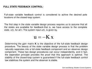
Pole Placement Problem Choose the state feedback gain to place the poles of the closed-loop system, i.e., At specified locations
State Feedback Control of a System in CCF Consider a SISO system in CCF: State Feedback Control
Closed-Loop CCF System Closed loop A matrix:
Choosing the Gain-CCF Closed-loop Characteristic Equation Desired Characteristic Equation: Control Gains:
Transformation to CCF To CCF Transform system Where x+(k)=x(k+1) (for simplicity) First, find how new state z1 is related to x:
Transformed State Equations Necessary Conditions for p: 0 0 0 1 Vector p can be found if the system is controllable:
State Transformation Invertibility State transformation: Matrix T is invertible since By the Cayley-Hamilton theorem.
Toeplitz Matrix The Cayley-Hamilton theorem can further be used to show that Matrix on the right is called Toeplitz matrix
State Transformation Formulas Formula 1: Formula 2:
State Feedback Control Gain Selection By Cayley Hamilton: or
Double Integrator-Matlab Solution T=0.5; lam=[0;0]; G=[1 T;0 1]; H=[T^2/2;T]; C=[1 0]; K=acker(G,H,lam); Gcl=G-H*K; clsys=ss(Gcl,H,C,0,T); step(clsys);
Flexible System Example Consider the linear mass-spring system shown below: x1 x2 Parameters: m1=m2=1Kg. K=50 N/m k u m2 m1 • Analyze PD controller based on a)x1, b)x2 • Design state feedback controller, place poles at
Collocated Control Transfer Function: PD Control: Root-Locus
Non-Collocated Control Transfer Function: PD Control: Root-Locus Unstable
State Model Discretized Model: x(k+1)=Gx(k)+Hu(k)
Open-Loop System Information Controllability matrix: Characteristic equation: |zI-G|=(z-1)2(z2-1.99z+1)=z4-3.99z3+5.98z2-3.99z+6
State Feedback Controller Characteristic Equations: |zI-G|=(z-1)2(z2-1.99z+1)=z4-3.99z3+5.98z2-3.99z+6
Matlab Solution %System Matrices m1=1; m2=1; k=50; T=0.01; syst=ss(A,B,C,D); A=[0 0 1 0;0 0 0 1;-50 50 0 0;50 -50 0 0]; B=[0; 0; 1; 0]; C=[1 0 0 0;0 1 0 0]; D=zeros(2,1); cplant=ss(A,B,C,D); %Discrete-Time Plant plant=c2d(cplant,T); [G,H,C,D]=ssdata(plant);
Matlab Solution %Desired Close-Loop Poles pc=[-20;-20;-5*sqrt(2)*(1+j);-5*sqrt(2)*(1-j)]; pd=exp(T*pc); % State Feedback Controller K=acker(G,H,pd); %Closed-Loop System clsys=ss(G-H*K,H,C,0,T); grid step(clsys,1)
Steady-State Gain Closed-loop system: x(k+1)=Gclx(k)+Hr(k), Y=Cx(k) Y(z)=C(zI-Gcl)-1H R(z) If r(k)=r.1(k) then yss=C(I-Gcl)-1H Thus if the desired output is constant r=yd/gain, gain= C(I-Gcl)-1H
Integral Control Control law: 1/g y x u yd Ki Z-1 C H G plant Integral controller -Ks Automatically generates reference input r!
Closed-Loop Integral Control System Plant: Control: Integral state: Closed-loop system
Double Integrator-Matlab Solution T=0.5; lam=[0;0;0]; G=[1 T;0 1]; H=[T^2/2;T]; C=[1 0]; Gbar=[G zeros(2,1);C 1]; Hbar=[H;0]; K=acker(Gbar,Hbar,lam); Gcl=Gbar-Hbar*K; yd=1; r=0; %unknown gain clsys=ss(Gcl,[H*r;-yd],[C 0;K],0,T); step(clsys);