FULL STATE FEEDBACK CONTROL:
FULL STATE FEEDBACK CONTROL:. Full-state variable feedback control is considered to achive the desired pole locations of the closed-loop system.

FULL STATE FEEDBACK CONTROL:
E N D
Presentation Transcript
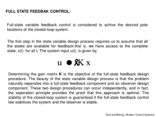
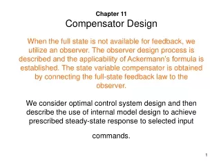
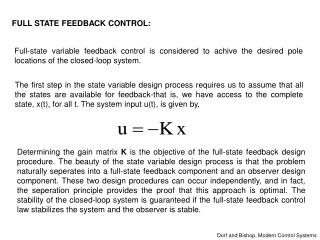
FULL STATE FEEDBACK CONTROL: Full-state variable feedback control is considered to achive the desired pole locations of the closed-loop system. The first step in the state variable design process requires us to assume that all the states are available for feedback-that is, we have access to the complete state, x(t), for all t. The system input u(t), is given by, Determining the gain matrix K is the objective of the full-state feedback design procedure. The beauty of the state variable design process is that the problem naturally seperates into a full-state feedback component and an observer design component. These two design procedures can occur independently, and in fact, the seperation principle provides the proof that this approach is optimal. The stability of the closed-loop system is guaranteed if the full-state feedback control law stabilizes the system and the observer is stable. Dorf and Bishop, Modern Control Systems
System Model x u Kontrol Law -K Full-state feedback The full-state feedback block diagram is illustrated in Figure 1. Figure 1. Full-state feedback block diagram (with no reference input)
With the system defined by the state variable model and the control feedback given by we find the closed-loop system to be The characteristic equation associated with above equation is If all the roots of the characteristic equation lie in the left-half plain, then the closed loop is stable. In other words, for any initial condition x(t0), it follows that Dorf and Bishop, Modern Control Systems
System Model u r(t) N x Kontrol Law -K Given the pair (A,B), we can always determine K to place all the system closed loop poles in the left half-plane if and only if the system is completely controllable-that is, if and only if the controllability matrix PC is full rank (for a SISO system, full rank implies that PC is invertible). The addition of a reference input can be considered as
Where r(t) is the reference input. When r(t)=0 for all t>t0, the control design problem is known as the regulator problem. That is, we desire to compute K so that all initial conditions are driven to zero in a desirable fashion (as determined by the design specifications). When using this state variable feedback, the roots of the characteristic equation are placed where the transient performance meets the desired response. Example: Consider the third-order system with the differential equation Dorf and Bishop, Modern Control Systems
We can select the state variables as x1=y, x2=dy/dt, x3=d2y/dt2. (Phase variables) and
If the state variable matrix is and then the closed-loop system is The state feedback matrix is Dorf and Bishop, Modern Control Systems
and the characteristic equation is clc;clear syms k1,k2,k3 mtrx=[0,1,0;0,0,1;(-2-k1),(-3-k2),(-5-k3)]; det(mtrx) If we seek a rapid response with a low overshoot, we choose a desired characteristic equation such that We choose ζ=0.8 for minimal overshoot and ωn to meet the settling time requirement.
If we want a settling time (with a 2% criterion) equal to 1 second, then If we choose ωn=6 rad/s, the desired characteristic equation is Comparing two characteristic equations yields Therefore, we require that k1=170.8, k2=79.1 and k3=9.4.
ACKERMANN’S FORMULA: For a single-input, single output system, Ackermann’s formula is useful for determining the state variable feedback matrix where Given the characteristic equation The state feedback gain matrix is where where PC is the controllability matrix.
Example: Consider the system and determine the feedback gain to place the closed-loop poles at s=-1±i. Therefore, we require that >>poly([-1+i -1-1i]) and α1= α2=2. With x1=y and x2=dy/dt, the matrix equation for the system G(s) is A B Dorf and Bishop, Modern Control Systems
The controllability matrix is Thus we obtain where and
k1 k2 Note that computing the gain matrix K using Ackermann’s formula requires the use of . We see that complete controllability is essential because only then we can guarantee that the controllabilty matrix PC has full rank and hence that exists. Then we have With Matlab >>A=[0 1;0 0]; >>B=[0;1]; >>K=acker(A,B,[-1+i,-1-i]) >>K=place(A,B,[-1+i,-1-i]) Result: K = 2 2 Dorf and Bishop, Modern Control Systems
OBSERVER DESIGN: In the full-state feedback design procedure discussed in the previous section, it was assumed that all the states were available for feedback at all times. This is a good assumption for the control law design process. However, generally speaking, only a subset of the states are readily measurable and available for feedback. Having all the states available for feedback implies that these states are measured with a sensor or sensor combinations. The cost and complexity of the control system increase as the number of required sensor increases. So, even in situations where extra sensors are available, it may not be cost-effective to employ these extra sensors, if indeed, the control system design goals can be accomplished without them. Fortunately, if the system is completely observable with a given set of outputs, then it is possible to determine (or estimate) the states that are not directly measured (or observed).
where denotes the estimate of the state x. The matrix L is the observer gain matrix and is to be determined as part of the observer design procedure. The observer is depicted in Figure 2. The observer has two inputs, u and y, and one output, . u y Observer + - C According to Luenberger, the full-state observer for the system is given by Figure 2. Observer. Dorf and Bishop, Modern Control Systems
The goal of the observer is to provide an estimate so that as t ∞. Remember that we do not know x(t0) precisely; therefore we must provide an initial estimate to the observer. Define the observer estimation error as The observer design should produce an observer with the property that e(t) 0 as t ∞. One of the main results of systems theory is that if the system is completely observable, we can always find L so that the tracking error is asymptotically stable, as desired. Taking the time-derivative of the estimation error in the error equation yields and using the system model and the observer, we obtain Dorf and Bishop, Modern Control Systems
or We can guarantee that e(t)0 as t∞ for any initial tracking error e(t0) if the characteristic equation has all its roots in the left half-plane. Therefore, the observer design process reduces to finding the matrix L such that the roots of the characteristic equation lie in the left half-plane. This can always be accomplished if the system is completely observable; that is, if the observability matrix, PO, has full rank. Example: Consider the second-order system
In this example, we can only directly observe the state y=x1. The observer will provide estimates of the second state, x2. The observer design begins by checking the system observability to verify that an observer can be constructed to guarantee the stability of the estimation error. From the system model, we find that The corresponding observability matrix Since det PO=3, the system is completely observable. Suppose that the desired charactersictic equation is given by
We can select ζ=0.8 and ωn=10, resulting in an expected settling time of less than 0.5 second. Computing the actual characteristic equation yields where Equating the coefficients yields the two equations which, when solved, produces Dorf and Bishop, Modern Control Systems which, when solved, produces
The observer is thus given by Dorf and Bishop, Modern Control Systems
Matlab Code clc;clear A=[-20 3;-60 4];B=[0;0];C=[0 0];D=[0]; sys=ss(A,B,C,D) %state-space model x0=[1 -2]; %initial conditions t=[0:0.01:1]; u=0*t; %zero input [y,T,x]=lsim(sys,u,t,x0); plot(T,x(:,1),T,x(:,2)) xlabel('Time (seconds)') The response of the estimation error to an initial error of is shown in the figure.
Ackermann’s formula can also be employed to place the roots of the observer characteristic equation at the desired locations. Consider the observer gain matrix and the desired observer characteristic equation The β’s are selected to meet given performance specifications for the observer. The observer gain matrix is then computed via where PO is the observability matrix Dorf and Bishop, Modern Control Systems
Example: Consider the second-order system given in previous example. The desired characteristic equation is given where ζ=0.8 and ωn=10, hence, β1=16 and β2=100. Computing p(A) yields We have the observability matrix which implies that
System model x u C y Observer + Conrol Law -K - C Compensator Using Ackermann’s formula yields the observer gain matrix COMPENSATOR DESIGN:INTEGRATED FULL-STATE FEEDBACK AND OBSERVER The state variable compensator is constructed by appropriately connecting the full-state feedback conrol law to the observer. The compensator is shown in Figure 3. Figure 3. State variable compensator employing full-state feedback in series with a full-state observer.
Our strategy was to design the state feedback control law as u(t)=-Kx(t), where we assumed that we had access to the complete state x(t). Then we designed an observer to provide an estimate of the state . It seems reasonable that we can employ the state estimate in the feedback control law in place of x(t). In other words, we can consider the feedback law The feedback gain matrix K was designed to guarantee stability of the closed-loop system; that is, the roots of the charactersitic equation are in the left-half plane. Under the assumption that the complete state x(t) is available for feedback, the feedback control law (with properly designed gain matrix K) leads to the desired results that x(t)0 as t ∞ for any initial condition x(t0). We need to verify that, when using the feedback control law for observed states, we retain the stability of the closed-loop system. Dorf and Bishop, Modern Control Systems
Consider the observer again Substituting the feedback law and rearranging terms in the observer yields the compensator system Notice that the system in the equation has the form of a state variable model with input y and output u as illustrated in Figure 3. Computing the estimation error using the compensator yields or Dorf and Bishop, Modern Control Systems
This is the same result as we obtained for the estimation error. The estimation error does not depend on the input as seen in the error equation, where input terms cancel. Recall that the underlying system model is given by Substituting the feedback law into the system model and with we obtain
Recall that our goal is to verify that, with , we retain stability of the closed-loop system and the observer. The characteristic equation associated with the matrix equation We can write the equations in matrix form So if the roots of det[λI-(A-BK)]=0 lie in the left half-plane, and if the roots of det [λI-(A-LC)]=0 lie in the left half-plane, then the overall system is stable. Therefore, employing the strategy of using the state estimates for the feedback is in fact a good strategy. The fact that the full-state feedback law and the observer can be designed independently is an illustration of the seperation principle. Dorf and Bishop, Modern Control Systems
The design procedure is summarized as follows • Determine K such that det[λI-(A-BK)]=0 has roots in the left-half plane and place the poles appropriately to meet the control system design specifications. The ability to place the poles arbitrarily in the complex plane is guaranteed if the system is completely controllable. • Determine L such that det[λI-(A-LC)]=0 has roots in the left-half plane and place the poles to achieve acceptable observer performance. The ability to place the poles arbitrarily in the complex plane is guaranteed if the system is completely observable. • Connect the observer to full-state feedback law using Dorf and Bishop, Modern Control Systems