Probability and Probability Distributions
350 likes | 744 Vues
Probability and Probability Distributions. ASW, Chapter 4-5 Skip sections 4.5, 5.5, 5.6. September 24, 2008. Conditional probabilities (ASW, 162-167). A conditional probability refers to the probability of an event A occurring, given that another event B has occurred.

Probability and Probability Distributions
E N D
Presentation Transcript
Probability and Probability Distributions ASW, Chapter 4-5 Skip sections 4.5, 5.5, 5.6 September 24, 2008
Conditional probabilities (ASW, 162-167) • A conditional probability refers to the probability of an event A occurring, given that another event B has occurred. • Notation: P(A B) • Read this as the “conditional probability of A given B” or the “probability of A given B.” • Conditional probabilities are especially useful in economic analysis because probabilities of an event differ, depending on other events occurring.
Formulae for conditional probabilities • The conditional probability of A given B is • The conditional probability of B given A is
Number of students by major and Excel skill level This table contains the same data as examined earlier, but reorganized as a table rather than in a tree diagram.
Examples of conditional probabilities from student survey • Probability that each major has low skill level? P(L MA) = P(L MA) / P(MA) = (2/46) / (6/46) = 2/6 = 0.333 P(L B) = 3 / 13 = 0.231 P(L E) = 0.500 P(L O) = 0.333 If a student has a high skill level is Excel, what is the probability his or her major is Business? Other? P(B H) = P(B H) / P(H) = (3/46) / (6/46) = 3/6 = 0.500 P(O H) = 0.167
Using conditional probabilities • “While four-day workweeks make some sense for the manufacturing sector, it’s much more challenging for service-based companies that have to be available for clients’ questions. Even on Fridays.” Source: The Globe and Mail, September 20, 2008, B18. • Parents who resided in the largest census metropolitan areas were more likely to have an adult child at home. For example, 41% of parent in Vancouver but only 17% of parent living in rural areas or small towns shared their house with at least one adult child. Source: “Parents with adult children living at home.” Statistics Canada, Canadian Social Trends, Spring 2006.
Sample of Saskatchewan residents • Random sample of 2,500 Saskatchewan residents from the Census of Canada, 2001 Public Use Microdata File, Individuals File. Obtained from the Internet Data Library System, through the University of Regina Data Library Services. • Subgroup selected was those with ages 30-64 years, wages and salaries greater than zero, and full-time jobs in the year 2000. • This resulted in a sample of 700 individuals.
Number of Saskatchewan residents with various levels of wages and salaries and schooling, 2000
Some conditional probabilities What is the conditional probability of $45,000 in wages and salaries given less than twelve years of schooling? Given 14-17 years of schooling? Given 18+ years? P(45+ <12) = P(45+ <12) / P(<12) = 21/ 128 = 0.164 P(45+ 14-17) = 82/ 230 = 0.357 P(45+ 18+) = 0.451 That is, chances of a high income increase with each higher level of schooling. What is the probability that someone with a middle level of income has 12-13 years of schooling? P(12-13 20-45) = P(12-1320-45) / P(<20-45) = 135/ 325 = 0.415
Conditional probabilities of various levels of wages and salaries, given years of schooling, n=700 Saskatchewan residents, 2000
Organizing cross-classification tables ASW use joint probability tables with joint and marginal probabilities. Study the example on pages 163-164. • Joint probabilities are the probabilities of the intersection of each pair of events in a cross-classification table. • Marginal probabilities are the probabilities of each of the events in the rows and columns of the table. Conditional probabilities can be computed from the numbers of cases, as reported in the cross-classification table, as in the examples shown above. I find this method more useful for the following analysis of independence and dependence.
Independent and dependent events (ASW, 166) Two events A and B are independent if P(A B) = P(A) or P(B A) = P(B). That is, the probability of one event is not altered by whether or not the other event occurs. If P(A B) = P(A), then P(B A) = P(B), and vice-versa. Two events A and B are dependent if P(A B) ≠ P(A) or P(B A) ≠ P(B). In this case, the occurrence of one event affects the probability of the other event.
Example of dependence Does the event of having low wages and salaries depend on having few years of schooling? If A is the event of having a low salary (<$20,000) and B is the event of having less than twelve years of schooling P(A B) = 38/128 = 0.297 P(A) = 177/700 = 0.253 And P(A B) > P(A) so the chance of having low wages and salaries is greater for those with the least amount of schooling, as compared with the whole sample. Also note in this case that P(B A) = 38/177 = 0.215 > 0.183 = P(B). This is an alternative way of checking for whether the events are dependent or independent.
Example of independence Are the events of having 12-13 years of schooling (A) and the event of having wages and salaries of $20-45,000 (B) dependent or independent? P(A B) = 135/325 = 0.415 P(A) = 291/700 = 0.416 So these two events are essentially independent of each other. Also note that P(B A) = 135/291 = 0.464 P(B) = 325/700 = 0.464 In this case, those with a middle level of schooling (12-13 years) and the middle category of income are similar to a cross-section of the whole sample.
Using dependence and independence Some authors have argued that parents in higher socio-economic positions may have a greater tendency to expect their children to be independent earlier than those with less education and income….However, the analysis…does not show support for these interpretations. Parents with a higher level of education were neither more not less likely than less well-educated parents to live with their adult children. Nor were parents with high personal income any less likely than those with lower personal income to provide accommodation for their children. Source: “Parents with adult children living at home.” Statistics Canada, Canadian Social Trends, Spring 2006.
Independence and dependence in economic analysis Is the price of wheat received by Saskatchewan farmers dependent on the weather in Russia? Is the chance of NAFTA being renegotiated dependent on the result of the U.S. presidential election? Is the consumption of table salt dependent on interest rates? Is it dependent on health fads?
Multiplication rule (ASW, 165) The multiplication rule can be used to compute the probability of the intersection of two events. P(A ∩ B) = P(A) P(B A) P(A ∩ B) = P(B) P(A B) But note that if events A and B are independent of each other, then P(B A) = P(B) and P(A B) = P(A), so that P(A ∩ B) = P(A) P(B)
Example of multiplication rule What is the probability of wages and salaries of $20-45,000 (A) and having 12-13 years of schooling (B)? Since we already know that A and B are independent, P(A) x P(B) = (325/700) x (291/700) = 0.193. Note that P(A ∩ B) = 135 / 700 = 0.193 from the table. What is the probability of wages and salaries of $45,000+ (C) and having 14-17 years of schooling (D)? In this case, we have not checked for independence, so use the full formula: P(C ∩ D) = P(C) P(D C) = (198/700)X(82/198) = 82/700 = 0.117
Using independence • Independent trials of an experiment: • Successive flips of a coin. • Many rolls of a die or a pair of dice. • Sale of a product to customers arriving at a retail store. • If a population is small and a case that is selected is not replaced before the next case is drawn, then successive drawings are dependent on each other. But if the population is large, successive draws do not alter the composition of the population. Thus, random selection of respondents from a large population produces independence of successive selections. When trials of an experiment are independent of each other, then the binomial probability distribution can be used to determine the probability of several occurrences of an event in many trials– ASW, section 5.4.
Random variables (ASW, 185) • A random variable is a numerical description of the outcome of an experiment. • Or, a random variable attaches a numerical value to each possible experimental outcome. • A random variable is often assigned an algebraic symbol such as x. • A random variable can be either discrete (countable number of possible values) or continuous (not countable or any numerical value with an interval). • Chapter 5 deals with discrete random variables. • Chapter 6 deals with continuous random variables.
Discrete random variables • Any random variable that has a finite number of possible values or a countably infinite number of possible values. • Examples: • The number of females in a sample of 3 persons selected from a large population that is half female and half male (x = 0, 1, 2, 3). • The sum of the faces shown when a pair of dice is rolled (x = 2, 3, 4, … , 12). • The number of customers at a restaurant at lunch (x = 0, 1, 2, 3, 4, 5, … , 45). To the maximum of the number of seats. • The number of unemployed workers in Saskatchewan reported by Statistics Canada each month (x = 0, 1, 2, … , 29,800). • The number of homeowners who have defaulted on mortgages in the United States during the last year.
Continuous random variables • Any random variable whose possible values cannot be counted is termed continuous. Alternatively, if the possible outcomes can take on any numerical value in an interval or set of intervals, the random variable is continuous. • Examples: • Number of kilometres goods are transported from a manufacturing plant to a warehouse. • Time taken to ship the goods. • Exchange rates for currencies. • Household income. • We will study the continuous uniform distribution and the normal distribution (bell curve) next week.
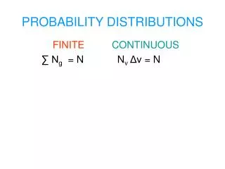
Probability distributions • A probability distribution is a random variable, along with the associated probabilities of occurrence of the values of the variable. • Discrete – probabilities of each value of the random variable. • Continuous – probability that the random variable is within a particular interval.
Discrete probability distribution. (ASW, 189-192) For a discrete random variable x, the probability distribution is the set of values of x, along with f(x), the function that gives the probability for each value of x. For each value of x, f(x) is no less than 0 and no greater than 1. The sum of the probabilities for all values of x equals 1. Symbolically, 0 f(x) 1 ∑ f(x) = 1
Probability distribution for sex of person selected Equally likely outcomes for experiment of randomly selecting 3 persons from a large population of half males and half females: FFF FFM FMF FMM MFF MFM MMF MMM Let the random variable x be the number of females selected and f(x) the probabilities for each value of x. In this example, the values of f(x) are obtained using the classical interpretation of probability.
Responses to “Would you like to lower tuition, even if it meant larger class sizes?
If a student is randomly selected, let x be the response to the lower tuition question. In this case, the values of the probability function f(x) are the relative frequencies of occurrence of the responses to the question. Probability distribution and expected value for lower tuition question
Graphing discrete probability distributions • Use a line chart as in Figure 5.1 of ASW. Or it could be a bar chart with spaces left between the bars, to visually indicate that it is a discrete distribution. • Convention is to place the values of the random variable x on the horizontal axis and values of the probability function f(x) on the vertical axis. • Examples that follow illustrate these methods.
Expected values (ASW, 195) The expected valueE(x) of a random variable x is the mean of the probability distribution. Symbolically, E(x) = μ = ∑ x f(x) where μ (pronounced something like “mu”) is a Greek symbol used to indicate mean. The concept of expected value is more general than just referring to the mean, in that the expected value can be obtained for other expressions – see later notes on the variance. However, in this course, it will be used to denote the expected value of x, or the mean.
Expected value for x, number of females selected E(x) = μ = ∑ x f(x) = 1.500 If a random sample of 3 persons is obtained from a large population composed of half females and half males, the expected number of females selected is 1.5. If there are many samples of 3 persons each time, the mean number of females across the samples is 1.5.
The expected value of the responses is 3.869, or 3.9. Recall that a response of 3 was “indifferent” and a response of 4 was “weak yes” so, in this sample, the expected value or mean is just below “weak yes.” Expected value for responses to lower tuition question
Variance (ASW, 195) The variance of a probability distribution is the expected value of the squares of the differences of the random variable x from the mean μ. Symbolically, Var(x) = σ2 = ∑(x – μ)2f(x) The Greek symbol σ is “sigma.” The variance can be difficult to calculate and interpret. It is in units that are the square of the random variable x. Partly because of this, in statistical work it is more common to use the square root of the variance or σ. The standard deviation has the same units as x.
Variance of x, number of females selected If a random sample of 3 persons is obtained from a large population composed of half females and half males, the expected number of females selected is μ = 1.5. The variance of the number of females selected is Var(x) = σ2 = ∑(x – μ)2f(x) = 0.75. The standard deviation is the square root of 0.75, so that σ = 0.866.
Later this class or next day • Binomial probability distribution • Continuous probability distributions • Bring along copies of the Normal Distribution for Monday and Wednesday, Sept. 29 and October 1. This is Table 1 of Appendix B of ASW.
