Probability Distributions
1.09k likes | 1.3k Vues
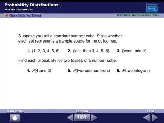
Probability Distributions. ALGEBRA 2 LESSON 12-1. (For help, go to Lesson 1-6.). Suppose you roll a standard number cube. State whether each set represents a sample space for the outcomes. 1. {1, 2, 3, 4, 5, 6} 2. {less than 3, 4, 5, 6} 3. {even, prime}

Probability Distributions
E N D
Presentation Transcript
Probability Distributions ALGEBRA 2 LESSON 12-1 (For help, go to Lesson 1-6.) Suppose you roll a standard number cube. State whether each set represents a sample space for the outcomes. 1. {1, 2, 3, 4, 5, 6} 2. {less than 3, 4, 5, 6} 3. {even, prime} Find each probability for two tosses of a number cube. 4.P(4 and 3) 5. P(two odd numbers) 6. P(two integers) 12-1
Solutions 1. {1, 2, 3, 4, 5, 6}; yes 2. {less than 3, 4, 5, 6} = {1, 2, 4, 5, 6}; no (3 is missing) 3. {even, prime} = {2, 4, 6, 3, 5}; no (1 is missing) 4. Sample space for two tosses of a number cube: P(4 and 3) = P(4 3 or 3 4) = = 5.P(two odd numbers) = P(1 1, 1 3, 1 5, 3 1, 3 3, 3 5, 5 1, 5 3, or 5 5) = = 6.P(two integers) = = 1 1 2 3 4 5 6 1 1 1 2 1 3 1 4 1 5 1 6 2 1 2 2 2 3 2 4 2 5 2 6 3 1 3 2 3 3 3 4 3 5 3 6 4 1 4 2 4 3 4 4 4 5 4 6 5 1 5 2 5 3 5 4 5 5 5 6 6 1 6 2 6 3 6 4 6 5 6 6 1 2 3 4 5 6 1 18 2 36 9 36 1 4 36 36 Probability Distributions ALGEBRA 2 LESSON 12-1 12-1
Below are three types of eye color: brown (BR), green (GR), and blue (BL). Make a frequency table. GR GR BR GR BR BR BR BL BR GR BR BR BL GR BR BR BR BL BL GR BR BR BR BR BR Step 1:Count the number of each type. Step 2:Make a table. Eye Color Number Brown 15 Green 6 Blue 4 Total 25 Brown IIII IIII IIII Green IIII I Blue IIII Total number of pairs of eyes: 25 Probability Distributions ALGEBRA 2 LESSON 12-1 Take a survey of your classmates’ eye colors and make a frequency table with the data. 12-1
More than one activity 144 One activity 360 No activities 216 Total Students 720 144 720 P(more than one activity) = Find the experimental probability for each event in the table that P(one activity) = represents at least one extra- curricular activity. 360 720 144 720 360 720 504 720 + = = 0.7 Add to find the cumulative probability. Probability Distributions ALGEBRA 2 LESSON 12-1 Use the frequency table. Find the probability that a student is involved in at least one extra-curricular activity. 12-1
Spinning two Spinners There are 16 possible outcomes. Divide to find the probability. Sum 2 3 4 5 6 7 8 Frequency 1 2 3 4 3 2 1 Probability 1 16 2 16 3 16 4 16 3 16 2 16 1 16 Probability Distributions ALGEBRA 2 LESSON 12-1 Suppose you spin two spinners. Each spinner has 4 possible outcomes: 1, 2, 3, or 4. Show the probability distribution for the sum of the numbers. Method 1: Make a frequency table. Then extend the table to include probabilities. Method 2: Draw a graph. 12-1
Parent Plant r r Parent R Rr Rr Plant r rr rr Probability Distributions ALGEBRA 2 LESSON 12-1 Use information in the chart of inherited gene pairs. Graph the probability distribution for each sample space. Inherited Gene Pairs From One Recessive and One Hybrid Pea Plant RR = dominant gene pair (red flower) Rr = hybrid gene pair (pink flower) rr = recessive gene pair (white flower) a. Genotype Distribution b. Plant Color Distribution {Rr, rr} {red, pink, white} 12-1
C 0 1 2 3 4 5 P(C) 0.05 0.15 0.25 0.3 0.2 0.05 Probability Distributions ALGEBRA 2 LESSON 12-1 The probability of an information desk at a community library receiving calls C each hour varies according to the following distribution. Use random numbers to predict the number of calls received during an eight-hour shift. Step 1: Define how the simulation will be done. Use random numbers. Assign numbers from 1 to 100 to the event’s based on the probability of each event. Use cumulative probabilities to help you assign the numbers. 12-1
Since P(0) = 0.05, assign 5 numbers to this outcome. There are 30 numbers from 46 to 75. Cumulative Assigned Outcome Probability Probability Numbers 0 0.05 0.05 01–05 1 0.15 0.20 06–20 2 0.25 0.45 21–45 3 0.30 0.75 46–75 4 0.20 0.95 76–95 5 0.05 1.00 96–100 Hour 1st 2nd 3rd 4th 5th 6th 7th 8th Random 95 91 15 52 41 74 5 34 numbers Number 4 4 1 3 2 3 0 2 of calls Probability Distributions ALGEBRA 2 LESSON 12-1 (continued) Step 2: Conduct the simulation. Model an eight-hour period by generating eight random numbers from 1 to 100. 12-1
Probability Distributions ALGEBRA 2 LESSON 12-1 (continued) To construct the table: Find the random number in the assigned numbers column, then assign the outcome as the number of calls. The random number 41 is assigned to the outcome of 2 calls. Step 3: Interpret the simulation. Based on this simulation, a total of 19 calls came into the information desk over an eight-hour period. 12-1
Probability Distributions ALGEBRA 2 LESSON 12-1 pages 639–641 Exercises 1. 2. 3. 0.11 4. 0.89 5. 0.53 6. 7. 12-1
> – Probability Distributions ALGEBRA 2 LESSON 12-1 10. Answers will vary. Sample design: Use random numbers. Assign numbers 1 to 1000 to each event, based on its probability. Cumulative Assigned Age Probability Probability Numbers < 20 0.051 0.051 1–51 20–29 0.176 0.227 52–227 30–39 0.211 0.438 228–438 40–49 0.211 0.649 439–649 50–59 0.156 0.805 650–805 60–69 0.096 0.901 806–901 70–79 0.070 0.971 902–971 80 0.029 1.000 972–1000 Random numbers generated: 697, 420, 488, 567, 272, 396, 474, 870, 896, 282, 464, 681, 274, 663, 681, 282, 376, 363, 860, 129 Results of simulation: Age 20–29: 1, Age 30–39: 8; Age 40–49: 4, Age 50–59: 4; Age 60–69: 3 8. 9. 12-1
Probability Distributions ALGEBRA 2 LESSON 12-1 11. Answers will vary. Sample design: Use random numbers. Assign numbers 1 to 1000 to each event, based on its probability. Assigned Type Prob. Cum. Prob. Numbers Luxury 0.165 0.165 1–165 Large 0.076 0.241 166–241 Midsize 0.527 0.768 242–768 Small 0.232 1 769–1000 Random numbers generated: 612, 904, 249, 194, 435, 772, 93, 236,80, 370, 849, 468, 819, 800, 371, 14, 396, 278, 303, 662, 637, 572, 700, 196, 810, 314, 496, 408, 737, 624 Results of simulation: 3 luxury cars, 3 large cars, 18 midsize cars, and 6 small cars 12. 13. 12-1
14.a. b. The independent variable is the type of weather. The dependent variable is the probability that a type of weather occurs. c. OR 0.359 15. Check students’ work. 16. a. The independent variable is the amount of gas in the tank; the dependent variable is the percent of people who fill their tanks when they have a given amount of gas. b. c. 0.28 or 28% 131 365 Probability Distributions ALGEBRA 2 LESSON 12-1 12-1
17. Answers may vary. Sample: Suppose the events in a probability distribution are not equally likely. By assigning the appropriate number of equally likely outcomes to each event, you can design a simulation that reflects the actual probabilities expected. 18. 19. Answers may vary. Sample: a. b. There were six hours in which 3 calls were received, and two in which 4 calls were received. A total of ten callers would have to wait. c. d. An additional response team would reduce the probability of having to wait from to , a considerable improvement. 10 47 2 47 10 47 Probability Distributions ALGEBRA 2 LESSON 12-1 12-1
20.a. 0.0000001, 0.16, 0.84 b. Check students’ work. c. Check students’ work. 21. C 22. I 23.[4] Since + + + = 1, such a spinneris possible. Divide the spinner into 12 equal parts. Label 1 part A, 2 parts B, 4 parts C, and 5 parts D. [3] incorrectly divides the 12 parts [2] does not explain answer [1] incorrectly adds probabilities 24. 3 units2 25. 4 units2 26. 2 units2 27. 28. 29. dependent 30. independent 5 12 2 12 1 6 1 3 Probability Distributions ALGEBRA 2 LESSON 12-1 12-1
Probability Distributions ALGEBRA 2 LESSON 12-1 1. During lunch on Monday, the cafeteria deli sold soft drinks to 32 customers, bottled waters to 12 customers, sandwiches to 16 customers, tacos to 12 customers, salads to 13 customers, and baked potatoes to 9 customers. There were a total of 50 customers during lunch on Monday. a. Make a frequency table for the data. Extend the table to include a probability distribution. b. What is the probability that the next customer will order a drink? 12-1
Ride per week P (rides per week) 0 0.52 1 0.25 2 0.13 3 0.08 4 or more 0.02 Probability Distributions ALGEBRA 2 LESSON 12-1 2. Given the data on the number of bus rides per week for 100 people surveyed, conduct a simulation for the number of bus rides per week for the next ten people surveyed. 12-1
Item Freq. Prob. Soft drinks 32 Bottled Water 12 Sandwiches 16 Tacos 12 Salads 13 Baked potatoes 9 Total customers 50 32 50 12 50 16 50 12 50 13 50 9 50 Probability Distributions ALGEBRA 2 LESSON 12-1 1. During lunch on Monday, the cafeteria deli sold soft drinks to 32 customers, bottled waters to 12 customers, sandwiches to 16 customers, tacos to 12 customers, salads to 13 customers, and baked potatoes to 9 customers. There were a total of 50 customers during lunch on Monday. a. Make a frequency table for the data. Extend the table to include a probability distribution. b. What is the probability that the next customer will order a drink? 0.88 12-1
Answers will vary. Sample: Use random numbers. Assign numbers from 1 to 100 to events based on the probability of each event. Ride per week P (rides per week) 0 0.52 1 0.25 2 0.13 3 0.08 4 or more 0.02 Person Surveyed 1 2 3 4 5 6 7 8 9 10 Random Numbers 40 19 91 92 92 33 38 52 74 4 Rides per week 0 0 3 3 3 0 0 0 1 0 Probability Distributions ALGEBRA 2 LESSON 12-1 2. Given the data on the number of bus rides per week for 100 people surveyed, conduct a simulation for the number of bus rides per week for the next ten people surveyed. 12-1
Conditional Probability ALGEBRA 2 LESSON 12-2 (For help, go to Lesson 9-7.) A spinner has four equal sections that are red, blue, green, and yellow. Find each probability for two spins. 1.P(blue, then blue) 2.P(red, then yellow) 3.P(not yellow, then green) 4.P(not blue, then not red) 5.P(at least one green) 6.P(neither spin red) 12-2
Solutions 1. P(blue, then blue) = P(blue) • P(blue) = • = 2.P(red, then yellow) = P(red) • P(yellow) = • = 3.P(not yellow, then green) = P(not yellow) • P(green) = • = 4.P(not blue, then not red) = P(not blue) • P(not red) = • = 1 4 1 4 1 16 1 16 1 4 1 4 3 4 1 4 3 16 3 4 3 4 9 16 Conditional Probability ALGEBRA 2 LESSON 12-2 12-2
R B G Y R B G Y R R R B R G R Y B R B B B G B Y G R G B G G G Y Y R Y B Y G Y Y Conditional Probability ALGEBRA 2 LESSON 12-2 Solutions (continued) 5. Sample space for two spins: P(at least one green) = P(R G, B G, G G, Y G, G R, G B, or G Y) = 6. See sample space in Exercise 5 above. P(neither spin red) = P(B B, B G, B Y, G B, G G, G Y, Y B, Y G, or Y Y) = 7 16 9 16 12-2
yes no female 8 6 male 5 7 Do you own a pet? 8 14 Therefore, P(own a pet | female) equals . Conditional Probability ALGEBRA 2 LESSON 12-2 The table shows the results of a class survey. Find P(own a pet | female) The condition female limits the sample space to 14 possible outcomes. Of the 14 females, 8 own a pet. 12-2
Material Recycled Not Recycled Paper 34.9 48.9 Metal 6.5 10.1 Glass 2.9 9.1 Plastic 1.1 20.4 Other 15.3 67.8 20.4 48.9 + 10.1 + 9.1 + 20.4 + 67.8 P(plastic | non-recycled) = 20.4 156.3 = 0.13 Conditional Probability ALGEBRA 2 LESSON 12-2 Using the data in the table, find the probability that a sample of not recycled waste was plastic. The given condition limits the sample space to non-recycled waste. A favorable outcome is non-recycled plastic. The probability that the non-recycled waste was plastic is about 13%. 12-2
Relate: P( male ) = 58% P( male and jogs ) = 20% Define: Let A = male. Let B = jogs. P( A and B ) P( A ) Write: P( A | B ) = 0.2 0.58 = Substitute 0.2 for P(A and B) and 0.58 for P(A). 0.344 Simplify. Conditional Probability ALGEBRA 2 LESSON 12-2 Researchers asked people who exercise regularly whether they jog or walk. Fifty-eight percent of the respondents were male. Twenty percent of all respondents were males who said they jog. Find the probability that a male respondent jogs. The probability that a male respondent jogs is about 34%. 12-2
Conditional Probability ALGEBRA 2 LESSON 12-2 Jim created the tree diagram after examining years of weather observations in his hometown. The diagram shows the probability of whether a day will begin clear or cloudy, and then the probability of rain on days that begin clear and cloudy. a. Find the probability that a day will start out clear, and then will rain. The path containing clear and rain represents days that start out clear and then will rain. P(clear and rain) = P(rain | clear) • P(clear) = 0.04 • 0.28 = 0.011 The probability that a day will start out clear and then rain is about 1%. 12-2
Conditional Probability ALGEBRA 2 LESSON 12-2 (continued) b. Find the probability that it will not rain on any given day. The paths containing clear and no rain and cloudy and no rain both represent a day when it will not rain. Find the probability for both paths and add them. P(clear and no rain) + P(cloudy and no rain) = P(clear) • P(no rain | clear) + P(cloudy) • P(no rain | cloudy) = 0.28(.96) + .72(.69) = 0.7656 The probability that it will not rain on any given day is about 77%. 12-2
Conditional Probability ALGEBRA 2 LESSON 12-2 pages 644–646 Exercises 1. 0.9 2. 0.6 3. 0.6 4. 0.085 5. 0.406 6. 0.529 7. 0.568 8. 0.780 9. 45% 10. 23% 11. 0.1, 0.114 12. P(W) = 0.55 13. a. 0.15 b. 0.60 c.P(A) is equal to P(A | B) d. The fact that P(A) = P(A | B) illustrates that the probability of A is the same, regardless of the occurrence of B. 12-2
Conditional Probability ALGEBRA 2 LESSON 12-2 14–18. Check students’ work. 19.P(C) 20.P(S and W) 21. P(R | W) 22.P(W | S) 23. a. The four right branches represent probabilities conditional upon the person being an adult or a minor. For example, the top branch represents the probability that a person is licensed given that he or she is an adult. b. No; the probability of a minor being licensed is not the same as the probability of an adult being licensed. c. Check students’ work. 24. P(I | N) = 0.2 25. C 26. H 27. D 12-2
< < < < – – – – 28.[2]P(B | A) = , where A is “the book is illustrated” and B is “the book is hardback”. 0.40 = 0.40 • P(A) = 0.20 P(A) = 0.5 [1] answer only OR minor error 29. 30. $492,000; $330,821 31. center (0, 0) x-intercepts (2, 0), (–2, 0) y-intercepts (0, 4), (0, –4); domain: {x|–2 x 2} range: {y|–4 y 4} 32. 2 33. 0.830 34. 1.404 35. 3.465 36. 0.1 37. 3.162 38. 49 P(A and B) P(A) > – 0.20 P(A) Conditional Probability ALGEBRA 2 LESSON 12-2 12-2
Conditional Probability ALGEBRA 2 LESSON 12-2 1. A study was conducted at Central High School to find out how much television students watch per night. Thirty-eight percent of the respondents were freshmen. Twenty-two percent of all respondents were freshmen who said that they watch at least one hour of television per night. Find the probability that a freshman respondent watches at least one hour of television per night. 2. The tree diagram below shows the probabilities that Jose will or will not cook breakfast on weekends (WE) or weekdays (WD). Find the probability that Jose will cook breakfast on any given day. about 58% about 38% 12-2
Analyzing Data ALGEBRA 2 LESSON 12-3 (For help, go to Lessons 1-1.) Order each set of values from least to greatest. Then find the middle value. 1. 0.2 0.3 0.6 1.2 0.7 0.9 0.8 2. 11 23 15 17 21 18 21 3. 7.8 2.6 3.9 15.6 9.1 11.7 10.4 4. 76 89 80 82 86 84 86 12-3
Analyzing Data ALGEBRA 2 LESSON 12-3 Solutions 1. 0.2, 0.3, 0.6, 0.7, 0.8, 0.9, 1.2; middle value = 0.7 2. 11, 15, 17, 18, 21, 21, 23; middle value = 18 3. 2.6, 3.9, 7.8, 9.1, 10.4, 11.7, 15.6; middle value = 9.1 4. 76, 80, 82, 84, 86, 86, 89; middle value = 84 12-3
x (78 + 87 + 84 + 75 + 80 + 98 + 78 + 95 + 72) 9 747 9 = = = 83 x Use the symbol to designate the mean. 72 75 78 78 80 84 87 95 98 Find the median and the mode by ordering the values numerically. ModeMedian Analyzing Data ALGEBRA 2 LESSON 12-3 Find the mean, median, and mode for these values: 78, 87, 84, 75, 80, 98, 78, 95, 72. The mean is 83, the median is 80, and the mode is 78. 12-3
Location J F M A M J J A S O N D Dauphin Island, Alabama 51 53 60 70 75 82 84 84 80 72 62 56 Step 2: Use the LIST feature to access the MATH menu. Find the mean. Analyzing Data ALGEBRA 2 LESSON 12-3 Using the data in the table, find the mean, median, and mode for the water temperatures in Dauphin Island, AL. Gulf of Mexico Eastern Coast Water Temperatures (°F) Step 1: Use the STAT feature to enter data as L1 in your graphing calculator. 12-3
Step 4: Use the STAT PLOT feature to access PLOT 1. Choose the histogram, L1, and Frequency 1 options. Then enter an appropriate viewing window. Step 5: Graph the data. Use the TRACE feature to move to the highest point of the graph. On the screen, the mode appears as the minimum value for the cursor. The mode is 84. The mode occurs two times in the data. Analyzing Data ALGEBRA 2 LESSON 12-3 (continued) Step 3: Return to the same menu to find the median. The mean is about 69.1°F, the median is 71°F, and the mode is 84°F. 12-3
Step 1: Find the quartile values, the minimum value, and the maximum value. 81 85 88 90 91 94 95 97 100 Q2 = median = 91 The median is a value of the data set, it is removed for the calculation of Q1 and Q3. 81 85 88 90 94 95 97 100 Q1 = = 86.5Q3 = = 96 (95 + 97) 2 (85 + 88) 2 Analyzing Data ALGEBRA 2 LESSON 12-3 Make a box-and-whisker plot for these values: 91, 95, 88, 85, 90, 97, 94, 100, 81. The minimum value is 81 and the maximum value is 100. 12-3
Step 3:Finish your box-and-whisker plot by drawing a box through Q1 and Q3, a vertical line through the median, and line segments from the box outward to the minimum and maximum values. Analyzing Data ALGEBRA 2 LESSON 12-3 (continued) Step 2: Draw a number line for the base of your box-and-whisker plot. Above the number line, plot the three quartiles, the minimum value, and the maximum value. 12-3
Use the STAT PLOT feature to select a box-and-whisker plot. Enter the window values. Graph the box-and-whisker plot. Analyzing Data ALGEBRA 2 LESSON 12-3 Use a graphing calculator to find the quartiles of the water temperature data for Dauphin, AL in Additional Example 2. Use the TRACE feature to find the quartile values. They are Q1 = 58, Q2 = 71, and Q3 = 81. 12-3
Analyzing Data ALGEBRA 2 LESSON 12-3 Find the 30th and 60th percentiles for the values below. 54 98 45 87 98 64 21 61 71 82 93 65 62 98 87 24 65 97 31 47 Step 1: Order the values. 21 24 31 45 47 54 61 62 64 65 65 71 82 87 87 93 97 98 98 98 Step 2: Find the number of values that fall below the 30th percentile and the number that fall below the 60th percentile. Of the 20, 30% should fall below the 30th percentile and 60% should fall below the 60th percentile. 20 30% = 20 0.30 = 6 Since 61 is greater than 6 values, 61 is at the 30th percentile. 20 60% = 20 0.60 = 12 Since 82 is greater than 12 values, 82 is at the 60th percentile. The value at the 30th percentile is 61 and the value at the 60th percentile is 82. 12-3
Order the data. 15 26 28 30 32 34 34 Find the differences between adjacent values. 11 2 2 2 2 0 Analyzing Data ALGEBRA 2 LESSON 12-3 Identify an outlier for this set of values: 15 34 28 32 30 26 34. 15 is substantially different, so 15 is an outlier. 12-3
Analyzing Data ALGEBRA 2 LESSON 12-3 pages 652–655 Exercises 1. 4.36, 3, 1 2. 338.5, 316, no mode 3. 600.3, 535.5, 499 4. 5. 6. 7. 8. 5896, 6381 9. 6, 18 10. 9.8 11. 0 12.a. 0% b. No; if there are an even number of items in a data set, the median may lie between data values. c. No; 50% of a data set will always lie at or below the median. 13.a. b. 38 c. The main effect of removing the outlier is a shortening of the long whisker. The median decreases from 8.5 to 8. 12-3
Analyzing Data ALGEBRA 2 LESSON 12-3 14. 103; this value lowers the mean. 15. 381; this value raises the mean. 16. 0th 17. 60th 18. Only 14 out of 20 values are below 89, so 89 is at the 70th percentile. For a number to be at the 100th percentile, 100% of the values must be below that number. That is impossible since a number cannot be less than itself. 19. a. 18.9, 19 b. No; none of the values is significantly less or greater than the others. c. Recent earthquakes have been more consistent in their numbers, with fewer light years as well as fewer extremely heavy years; this is indicated by the shorter whiskers on the box-and-whisker plot for 1991 through 2000. 20. The median is a better representation for the data; a few outliers can heavily influence the mean without drastically affecting the median. 12-3
Analyzing Data ALGEBRA 2 LESSON 12-3 21.a. men’s: 13.02, women’s: 13.74 b. c. Answers may vary. Sample: The range for women’s shot put is greater than men’s. The men are more consistent, as indicated by the shorter box and whiskers. Overall the men tend to throw farther, with the men’s median equal to the women’s third quartile 22.a. b. A Presidential election greatly increases voter turnout rate for the House of Representatives. The median turnout increases by 12.9%. The minimum turnout in a Presidential election year is 6.9% greater than the maximum turnout for a non-Presidential election year. 23. D 24. G 12-3
Analyzing Data ALGEBRA 2 LESSON 12-3 29. yes; –9 30. yes; 17 31. no 32. yes; 0 33. 34. 25.[2] Order the 80 scores from lowest to highest. The 20th percentile is the score that is greater than 20%, or 16, of the values; the 60th percentile is the score that is greater than 60%, or 48, of the values. [1] minor error 26.[4] [3] 4 correct values out of 5 [2] 3 correct values [1] 1 correct value 27. 0.20 28. 0.56 12-3
Analyzing Data ALGEBRA 2 LESSON 12-3 1. Marina has the following quiz grades in her Algebra 2 class: 84, 90, 96, 100, 67, 88, 90, 92, 94. a. Find the mean, median, and mode for Marina’s quiz grades. b. Make a box-and-whisker plot for Marina’s grades. 2. Find the values at the 40th and 70th percentiles for the values below. 26, 37, 18, 45, 20, 36, 22, 25, 50, 41 3. Identify an outlier for this set of data: 65, 70, 56, 45, 59, 67, 62. 89; 90; 90 26; 41 45 12-3
Simplify each expression. Round your answer to the nearest hundredth. 1.2. 3. 8.4 • 1.25 4. 12 – 6 • 0.5 5. [(2 – 6)2 + (7 – 6)2 + (8 – 6)2] 6. (4 – 3)2 + (5 + 3)2 6 2.4 34.3 7 1 3 1 2 Standard Deviation ALGEBRA 2 LESSON 12-4 (For help, go to Skills Handbook page 845.) 12-4
Standard Deviation ALGEBRA 2 LESSON 12-4 Solutions 34.3 7 1. = 34.3 ÷ 7 = 4.9 2. = 6 ÷ 2.4 = 2.5 3. 8.4 • 1.25 = 10.5 4. 12 – 6 • 0.5 = 12 – 3 = 9 5. [(2 – 6)2 + (7 – 6)2 + (8 – 6)2] = [(–4)2 + 12 + 22] = [16 + 1 + 4] = [21] = 7 6. (4 – 3)2 + (5 + 3)2 = • 12 + 82 = + 64 8.03 6 2.4 1 3 1 3 1 3 1 3 1 2 1 2 1 2 12-4
medianFind the median. 16 16 17 192022 24 25 26 (16 + 17) 2 (24 + 25) 2 Q1 = = 16.5Q3 = = 24.5Find Q1 and Q3. Standard Deviation ALGEBRA 2 LESSON 12-4 There are 9 members of the Community Youth Leadership Board. Find the range and interquartile range of their ages: 22, 16, 24, 17, 16, 25, 20, 19, 26. greatest value – least value = 26 – 16 Find the range. = 10 Q3 – Q1 = 24.5 – 16.5 Find the interquartile range. = 8 The range is 10 years. The interquartile range is 8 years. 12-4
x = = 91 Find the mean. (78.2 + 90.5 + 98.1 +93.7 +94.5) 5 x x x – x (x – x)2 Organize the next steps in a table. 78.2 91 –12.8 163.84 90.5 91 –0.5 .25 98.1 91 7.1 50.41 93.7 91 2.7 7.29 94.5 91 3.5 12.25 = Find the standard deviation. (x – x)2 n 234.04 5 = 6.8 Standard Deviation ALGEBRA 2 LESSON 12-4 Find the mean and the standard deviation for the values 78.2, 90.5, 98.1, 93.7, 94.5. The mean is 91, and the standard deviation is about 6.8. 12-4
