Probability Distributions
This comprehensive overview of probability distributions covers essential definitions and concepts related to variables, random variables, and their classifications. It distinguishes between discrete and continuous random variables, explaining their characteristics and how they relate to probability functions. The document also explores cumulative distribution functions, mathematical expectations, variance, and standard deviation. Through examples, it illustrates how to calculate expected values and variances, emphasizing the significance of these calculations in solving probability problems.

Probability Distributions
E N D
Presentation Transcript
D E F I N I T I O N S Variable: A variable is an entity that can assume multiple values. Random Variable: A random variable is a variable that takes on different values based on chance. In other words, there are probabilities associated with the possible values of the variable (i.e. a random variable has an associated probability distribution).
D E F I N I T I O N S continued Discrete Random Variable: A discrete random variable is a random variable that can only assume certain discrete values. There may be a finite number of possible values, or the number of possible values may be countably infinite. These are characterized by a probability mass function. Continuous Random Variable: A continuous random variable is a random variable that can assume any of the values in an interval. The probabilities are associated with subintervals inside the interval over which the random variable is defined. For a continuous random variable, the probability of a point is zero. These are characterized by probability density functions.
D E F I N I T I O N S continued Cumulative Distribution Function: A cumulative distribution function is a formula (or a table) that may be used to obtain the probability of obtaining a value of the associated random variable that is less than or equal to a specific value of the random variable. The probability values for such a function range from 0 to 1.
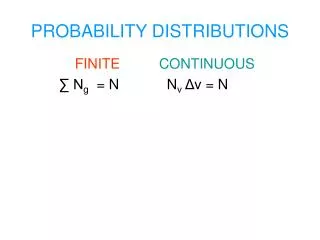
D I S C R E T E Let X be a discrete random variable. Then, 1) P(X) 0 for all values which are defined for X. 2) P(X) = 1 x C O N T I N U O U S Let X be a continuous random variable. Then, 1) P(a X b) 0 for any subinterval, [a,b], on which X is defined and a < b. P(X=a) = 0. 2) P(X) dx = 1 x P R O P E R T I E S O F P R O B A B I L I T Y D I S T R I B U T I O N S
MATHEMATICAL EXPECTATION The “Concept” Let X be a discrete random variable. The expected value of the random variable is the "average" of the values of X that would occur over many trials.
Point: A discrete random variable, x, has an associated probability function, P(x). The expected value of the random variable is also called the mean of the distribution and is denoted by . Definition: Let x be some discrete random variable with the probability function, P(x), then the expected value of x, denoted E(x), is defined: E(x) = xP(x) x
An Example Let x = the sum of the top faces when two dice are rolled. Let Di = the value on the top face of die i. The sample space is given by: D1: 1 1 1 1 1 1 2 2 2 2 2 2 3 3 3 3 3 3 4 4 4 4 4 4 5 5 5 5 5 5 6 6 6 6 6 6 D2: 1 2 3 4 5 6 1 2 3 4 5 6 1 2 3 4 5 6 1 2 3 4 5 6 1 2 3 4 5 6 1 2 3 4 5 6 If you compute all 36 sums, you will find there are: 1 sum of 2; 2 sums of 3; 3 sums of 4; 4 sums of 5; 5 sums of 6;1 sum of 12; 2 sums of 11; 3 sums of 10; 4 sums of 9; 5 sums of 8; and 6 sums of 7.
Probability Distribution Therefore, the probability distribution of x is: x P(x) 2 1/36 3 2/36 4 3/36 5 4/36 6 5/36 7 6/36 8 5/36 9 4/36 10 3/36 11 2/36 12 1/36
Expected Value of x, the mean E(x) = xP(x) x = 2(1/36) + 3(2/36) + 4(3/36) + 5(4/36) + 6(5/36) + 7(6/36) + 8(5/36) + 9(4/36) + 10(3/36) + 11(2/36) + 12(1/36) = 2 + 6 + 12 + 20 + 30 + 42 + 40 + 36 + 30 + 22 + 12 36 = 252/36 = 7. Therefore, = 7.
Variance of the distribution The variance of a distribution (2 ) is defined as the expected value of the squares of the deviations from the mean. Like before, the standard deviation () is the square root of the variance. Definition: Let x be some discrete random variable with the probability function, P(x), then the variance of x, denoted 2 = E[(x-)2], is defined: E[(x-)2] = (x-)2P(x) x
For our example 2 = (2-7)2(1/36) + (3-7)2(2/36) + (4-7)2(3/36) + (5-7)2(4/36) + (6-7)2(5/36) + (7-7)2(6/36) + (8-7)2(5/36) + (9-7)2(4/36) + (10-7)2(3/36) + (11-7)2(2/36) + (12-7)2(1/36) = 25 + 32 + 27 + 16 + 5 + 0 + 5 + 16 + 27 + 32 + 25 36 = 210/36 = 5.83. Therefore, 2.415229457
Q: Why would anyone want to go to this amount of trouble to calculate the mean and the standard deviation of a probability distribution? A: To approximate the solution of probability problems. True, it is a “pain” to calculate the mean and the variance of a distribution strictly from the definition, but usually it is not this much trouble, because there are “special cases” that are fairly simple calculations.
Special Discrete Probability Distributions • Hypergeometric • Binomial • Poisson

