B-Spline Blending Functions
B-Spline Blending Functions. The recurrence relation starts with the 1st order B-splines, just boxes, and builds up successively higher orders This algorithm is the Cox - de Boor algorithm Carl de Boor is in the CS department here at Madison. Uniform Cubic B-splines.

B-Spline Blending Functions
E N D
Presentation Transcript
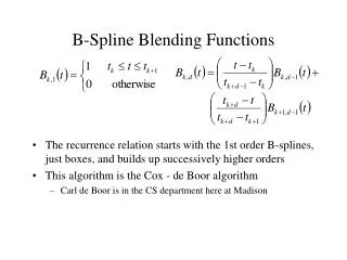
B-Spline Blending Functions • The recurrence relation starts with the 1st order B-splines, just boxes, and builds up successively higher orders • This algorithm is the Cox - de Boor algorithm • Carl de Boor is in the CS department here at Madison
Uniform Cubic B-splines • Uniform cubic B-splines arise when the knot vector is of the form (-3,-2,-1,0,1,…,n+1) • Each blending function is non-zero over a parameter interval of length 4 • All of the blending functions are translations of each other • Each is shifted one unit across from the previous one • Bk,d(t)=Bk+1,d(t+1) • The blending functions are the result of convolving a box with itself d times, although we will not use this fact
Uniform Cubic B-spline Blending Funcs B0,4 B1,4 B2,4 B3,4 B4,4 B5,4 B6,4
Computing the Curve P1B1,4 P4B4,4 P0B0,4 P2B2,4 P6B6,4 P3B3,4 P5B5,4
Using Uniform B-splines • At any point t along a piecewise uniform cubic B-spline, there are four non-zero blending functions • Each of these blending functions is a translation of B0,4 • Consider the interval 0t<1 • We pick up the 4th section of B0,4 • We pick up the 3rd section of B1,4 • We pick up the 2nd section of B2,4 • We pick up the 1st section of B3,4
Blending Function on [0,1] B1,4 B2,4 B0,4 B3,4
Uniform B-spline on [0,1) • Four control points are required to define the curve for 0t<1 • The blending functions sum to one, and are positive everywhere • The curve lies inside its convex hull • Does the curve interpolate its endpoints? • Look at the blending functions to decide • There is also a matrix form for the curve:
Uniform B-spline at Arbitrary t • The interval from an integer parameter value i to i+1 is essentially the same as the interval from 0 to 1 • The parameter value is offset by i • A different set of control points is needed • To evaluate a uniform cubic B-spline at an arbitrary parameter value t: • Find the greatest integer less than or equal to t: i = floor(t) • Evaluate: • Valid parameter range: 0t<n-3, where n is the number of control points
Loops • To create a loop, use control points from the start of the curve when computing values at the end of the curve: • Any parameter value is now valid • Although for numerical reasons it is sensible to keep it within a small multiple of n
B-splines and Interpolation, Continuity • Uniform B-splines do not interpolate control points, unless: • You repeat a control point three times • But then all derivatives also vanish (=0) at that point • To do interpolation with non-zero derivatives you must use non-uniform B-splines with repeated knots • To align tangents, use double control vertices • Then tangent aligns similar to Bezier curve • Uniform B-splines are automatically C2 • All the blending functions are C2, so sum of blending functions is C2 • Provides an alternate way to define blending functions • To reduce continuity, must use non-uniform B-splines with repeated knots
Rendering B-splines • Same basic options as for Bezier curves • Evaluate at a set of parameter values and join with lines • Hard to know where to evaluate, and how pts to use • Use a subdivision rule to break the curve into small pieces, and then join control points • What is the subdivision rule for B-splines? • Instead of subdivision, view splitting as refinement: • Inserting additional control points, and knots, between the existing points • Useful not just for rendering - also a user interface tool • Defined for uniform and non-uniform B-splines by the Oslo algorithm
Refining Uniform Cubic B-splines • Basic idea: Generate 2n-3 new control points: • Add a new control point in the middle of each curve segment: P’0,1, P’1,2, P’2,3 , …, P’n-2,n-1 • Modify existing control points: P’1, P’2, …, P’n-2 • Throw away the first and last control • Rules: • If the curve is a loop, generate 2n new control points by averaging across the loop • When drawing, don’t draw the control polygon, join the X(i) points
Rational Curves • Each point is the ratio of two curves • Just like homogeneous coordinates: • NURBS: x(t), y(t), z(t) and w(t) are non-uniform B-splines • Advantages: • Perspective invariant, so can be evaluating in screen space • Can perfectly represent conic sections: circles, ellipses, etc • Piecewise cubic curves cannot do this
OpenGL and Parametric Curves • OpenGL defines evaluators that evaluate a Bezier curve at a point • You give it the control points: • glMap1f(…) • Access a specific point: • glEvalCoord(param) • Access a sequence: • glMapGrid1f(n, t1,t2) • glEvalMesh1f(mode, p1, p2) • These functions evaluate the curve at equally spaced points - the poor way of drawing! • In hardware? Not yet, it seems.
OpenGL and NURBS • NURBS: Non-uniform Rational B-splines • The curved surface of choice in CAD packages • Support routines are part of the GLu utility library • Allows you to specify how they are rendered: • Can use points constantly spaced in parametric space • Can use various error tolerances - the good way! • Allows you to get back the lines that would be drawn • Allows you to specify trim curves • Only for surfaces (next lecture) • Cut out parts of the surface - in parametric space
From B-spline to Bezier • Both B-spline and Bezier curves represent cubic curves, so either can be used to go from one to the other • Recall, a point on the curve can be represented by a matrix equation: • P is the column vector of control points • M depends on the representation: MB-spline and MBezier • T is the column vector containing: t3, t2, t, 1 • By equating points generated by each representation, we can find a matrix MB-spline->Bezier that converts B-spline control points into Bezier control points