(Spline, Bezier, B-Spline)
1.26k likes | 3.2k Vues
(Spline, Bezier, B-Spline). Spline . Drafting terminology Spline is a flexible strip that is easily flexed to pass through a series of design points (control points) to produce a smooth curve.

(Spline, Bezier, B-Spline)
E N D
Presentation Transcript
Spline • Drafting terminology • Spline is a flexible strip that is easily flexed to pass through a series of design points (control points) to produce a smooth curve. • Spline curve – a piecewise polynomial (cubic) curve whose first and second derivatives are continuous across the various curve sections.
Bezier curve • Developed by Paul de Casteljau (1959) and independently by Pierre Bezier (1962). • French automobil company – Citroen & Renault. P1 P2 P3 P0
Parametric function n • P(u) = Bn,i(u)pi Where Bn,i(u) = . n!. ui(1-u)n-i i!(n-i)! 0<= u<= 1 i=0 For 3 control points, n = 2 P(u) = (1-u)2p0 + 2u(1-u) p1+ u2p2 For four control points, n = 3 P(u) = (1-u)3p0 + 3u(1-u) 2 p1 + 3u 2 (1-u)p2 + u3p3
01 21 11 10 00 20 algorithm • De Casteljau • Basic concept • To choose a point C in line segment AB such that C divides the line segment AB in a ratio of u: 1-u C A B P1 Let u = 0.5 u=0.25 u=0.75 P2 P0
properties • The curve passes through the first, P0 and last vertex points, Pn . • The tangent vector at the starting point P0 must be given by P1 – P0 and the tangent Pn given by Pn – Pn-1 • This requirement is generalized for higher derivatives at the curve’s end points. E.g 2nd derivative at P0 can be determined by P0 ,P1 ,P2 (to satisfy continuity) • The same curve is generated when the order of the control points is reversed
Properties (continued) • Convex hull • Convex polygon formed by connecting the control points of the curve. • Curve resides completely inside its convex hull
B-Spline • Motivation (recall bezier curve) • The degree of a Bezier Curve is determined by the number of control points • E. g. (bezier curve degree 11) – difficult to bend the "neck" toward the line segment P4P5. • Of course, we can add more control points. • BUT this will increase the degree of the curve increase computational burden
B-Spline • Motivation (recall bezier curve) • Joint many bezier curves of lower degree together (right figure) • BUT maintaining continuity in the derivatives of the desired order at the connection point is not easy or may be tedious and undesirable.
B-Spline • Motivation (recall bezier curve) – moving a control point affects the shape of the entire curve- (global modification property) – undesirable. • Thus, the solution is B-Spline – the degree of the curve is independent of the number of control points • E.g - right figure – a B-spline curve of degree 3 defined by 8 control points
B-Spline • In fact, there are five Bézier curve segments of degree 3 joining together to form the B-spline curve defined by the control points • little dots subdivide the B-spline curve into Bézier curve segments. • Subdividing the curve directly is difficult to do so, subdivide the domain of the curve by points called knots 0 u 1
B-Spline • In summary, to design a B-spline curve, we need a set of control points, a set of knots and a degree of curve.
B-Spline curve n • P(u) = Ni,k(u)pi (u0 < u < um).. (1.0) Where basis function = Ni,k(u) Degree of curve k-1 Control points, pi 0 < i < n Knot, u u0 < u < um m = n + k i=0
B-Spline : definition • P(u) = Ni,k(u)pi (u0 < u < um) • ui knot • [ui, ui+1) knot span • (u0, u1, u2, …. um ) knot vector • The point on the curve that corresponds to a knot ui, knot point ,P(ui) • If knots are equally space uniform (e.g, 0, 0.2, 0.4, 0.6…) • Otherwise non uniform (e.g: 0, 0.1, 0.3, 0.4, 0.8 …)
B-Spline : definition • Uniform knot vector • Individual knot value is evenly spaced • (0, 1, 2, 3, 4) • Then, normalized to the range [0, 1] • (0, 0.25, 0.5, 0.75, 1.0)
Type of B-Spline uniform knot vector Non-periodic knots (open knots) Periodic knots (non-open knots) • First and last knots are duplicated k times. • E.g (0,0,0,1,2,2,2) • Curve pass through the first and last control points • First and last knots are not duplicated – same contribution. • E.g (0, 1, 2, 3) • Curve doesn’t pass through end points. • used to generate closed curves (when first = last control points)
(Closed knots) Type of B-Spline knot vector Non-periodic knots (open knots) Periodic knots (non-open knots)
Non-periodic (open) uniform B-Spline • The knot spacing is evenly spaced except at the ends where knot values are repeated k times. • E.g P(u) = Ni,k(u)pi (u0 < u < um) • Degree = k-1, number of control points = n + 1 • Number of knots = m + 1 @ n+ k + 1 for degree = 1 and number of control points = 4 (k = 2, n = 3) Number of knots = n + k + 1 = 6 non periodic uniform knot vector (0,0,1,2,3, 3) * Knot value between 0 and 3 are equally spaced uniform n i=0
Non-periodic (open) uniform B-Spline • Example • For curve degree = 3, number of control points = 5 • k = 4, n = 4 • number of knots = n+k+1 = 9 • non periodic knots vector = (0,0,0,0,1,2,2,2) • For curve degree = 1, number of control points = 5 • k = 2, n = 4 • number of knots = n + k + 1 = 7 • non periodic uniform knots vector = (0, 0, 1, 2, 3, 4, 4)
0 0 i < k i – k + 1 k i n n – k + 2 n < i n+k ui = 0 0 i < 2 i – 2 + 1 2 i 3 3 – 2 + 2 3 < i 5 ui = Non-periodic (open) uniform B-Spline • For any value of parameters k and n, non periodic knots are determined from (1.3) e.g k=2, n = 3 u = (0, 0, 1, 2, 3, 3)
B-Spline basis function (1.1) (1.2) Otherwise • In equation (1.1), the denominators can have a value of zero, 0/0 is presumed to be zero. • If the degree is zero basis function Ni,1(u) is 1 if u is in the i-th knot span [ui, ui+1).
B-Spline basis function • For example, if we have four knots u0 = 0, u1 = 1, u2 = 2 and u3 = 3, knot spans 0, 1 and 2 are [0,1), [1,2), [2,3) • the basis functions of degree 0 are N0,1(u) = 1 on [0,1) and 0 elsewhere, N1,1(u) = 1 on [1,2) and 0 elsewhere, and N2,1(u) = 1 on [2,3) and 0 elsewhere. • This is shown below
B-Spline basis function • To understand the way of computing Ni,p(u) for p greater than 0, we use the triangular computation scheme
Non-periodic (open) uniform B-Spline Example • Find the knot values of a non periodic uniform B-Spline which has degree = 2 and 3 control points. Then, find the equation of B-Spline curve in polynomial form.
Non-periodic (open) uniform B-Spline Answer • Degree = k-1 = 2 k=3 • Control points = n + 1 = 3 n=2 • Number of knot = n + k + 1 = 6 • Knot values u0=0, u1=0, u2=0, u3=1,u4=1,u5= 1
Non-periodic (open) uniform B-Spline • Answer(cont) • To obtain the polynomial equation, P(u) = Ni,k(u)pi • = Ni,3(u)pi • = N0,3(u)p0 + N1,3(u)p1 + N2,3(u)p2 • firstly, find the Ni,k(u) using the knot value that shown above, start from k =1 to k=3 n i=0 2 i=0
Non-periodic (open) uniform B-Spline • Answer (cont) • For k = 1, find Ni,1(u) – use equation (1.2): • N0,1(u) = 1 u0 u u1 ; (u=0) • 0 otherwise • N1,1(u) = 1 u1 u u2 ; (u=0) • 0 otherwise • N2,1(u) = 1 u2 u u3 ; (0 u 1) • 0 otherwise • N3,1(u) = 1 u3 u u4 ; (u=1) • 0 otherwise • N4,1(u) = 1 u4 u u5 ; (u=1) • 0 otherwise
Non-periodic (open) uniform B-Spline • Answer (cont) • For k = 2, find Ni,2(u) – use equation (1.1): • N0,2(u) = u - u0 N0,1 + u2 – u N1,1 (u0 =u1 =u2 = 0) • u1 - u0 u2 – u1 • = u – 0 N0,1 + 0 – u N1,1 = 0 • 0 – 0 0 – 0 • N1,2(u) = u - u1 N1,1 + u3 – u N2,1 (u1 =u2 = 0, u3 = 1) • u2 - u1 u3 – u2 • = u – 0 N1,1 + 1 – u N2,1 = 1 - u • 0 – 0 1 – 0
Non-periodic (open) uniform B-Spline • Answer (cont) • N2,2(u) = u – u2 N2,1 + u4 – u N3,1 (u2 =0, u3 =u4 = 1) • u3 – u2 u4 – u3 • = u – 0 N2,1 + 1 – u N3,1 = u • 1 – 0 1 – 1 • N3,2(u) = u – u3 N3,1 + u5 – u N4,1 (u3 =u4 = u5 = 1) • u4 – u3 u5– u4 • = u – 1 N3,1 + 1 – u N4,1 = 0 • 1 – 1 1 – 1
Non-periodic (open) uniform B-Spline Answer (cont) For k = 2 N0,2(u) = 0 N1,2(u) = 1 - u N2,2(u) = u N3,2(u) = 0
Non-periodic (open) uniform B-Spline • Answer (cont) • For k = 3, find Ni,3(u) – use equation (1.1): • N0,3(u) = u - u0 N0,2 + u3 – u N1,2 (u0 =u1 =u2 = 0, u3 =1 ) • u2 - u0 u3 – u1 • = u – 0 N0,2 + 1 – u N1,2 = (1-u)(1-u) = (1- u)2 • 0 – 0 1 – 0 • N1,3(u) = u - u1 N1,2 + u4 – u N2,2 (u1 =u2 = 0, u3 = u4 = 1) • u3 - u1 u4 – u2 • = u – 0 N1,2 + 1 – u N2,2 = u(1 – u) +(1-u)u = 2u(1-u) • 1 – 0 1 – 0
Non-periodic (open) uniform B-Spline • Answer (cont) • N2,3(u) = u – u2 N2,2 + u5 – u N3,2 (u2 =0, u3 =u4 = u5 =1) • u4 – u2 u5 – u3 • = u – 0 N2,2 + 1 – u N3,2 = u2 • 1 – 0 1 – 1 • N0,3(u) =(1- u)2, N1,3(u) = 2u(1-u), N2,3(u) = u2 • The polynomial equation, P(u) = Ni,k(u)pi • P(u) = N0,3(u)p0 + N1,3(u)p1 + N2,3(u)p2 • = (1- u)2 p0 + 2u(1-u) p1 + u2p2 (0 <= u <= 1) n i=0
Non-periodic (open) uniform B-Spline • Exercise • Find the polynomial equation for curve with degree = 1 and number of control points = 4
Non-periodic (open) uniform B-Spline • Answer • k = 2 , n = 3 number of knots = 6 • Knot vector = (0, 0, 1, 2, 3, 3) • For k = 1, find Ni,1(u) – use equation (1.2): • N0,1(u) = 1 u0 u u1 ; (u=0) • N1,1(u) = 1 u1 u u2 ; (0 u 1) N2,1(u) = 1 u2 u u3 ; (1 u 2) • N3,1(u) = 1 u3 u u4 ; (2 u 3) N4,1(u) = 1 u4 u u5 ; (u=3)
Non-periodic (open) uniform B-Spline • Answer (cont) • For k = 2, find Ni,2(u) – use equation (1.1): • N0,2(u) = u - u0 N0,1 + u2 – u N1,1 (u0 =u1 =0, u2 = 1) • u1 - u0 u2 – u1 • = u – 0 N0,1 + 1 – u N1,1 • 0 – 0 1 – 0 • = 1 – u (0 u 1)
Non-periodic (open) uniform B-Spline • Answer (cont) • For k = 2, find Ni,2(u) – use equation (1.1): • N1,2(u) = u - u1 N1,1 + u3 – u N2,1 (u1 =0, u2 =1, u3 = 2) • u2 - u1 u3 – u2 • = u – 0 N1,1 + 2 – u N2,1 • 1 – 0 2 – 1 • N1,2(u) = u (0 u 1) • N1,2(u) = 2 – u (1 u 2)
Non-periodic (open) uniform B-Spline • Answer (cont) • N2,2(u) = u – u2 N2,1 + u4 – u N3,1 (u2 =1, u3 =2,u4 = 3) • u3 – u2 u4 – u3 • = u – 1 N2,1 + 3 – u N3,1 = • 2 – 1 3 – 2 • N2,2(u) = u – 1 (1 u 2) • N2,2(u) = 3 – u (2 u 3)
Non-periodic (open) uniform B-Spline • Answer (cont) • N3,2(u) = u – u3 N3,1 + u5 – u N4,1 (u3 = 2, u4 = 3, u5 = 3) • u4 – u3 u5– u4 • = u – 2 N3,1 + 3 – u N4,1 = • 3 – 2 3 – 3 • = u – 2 (2 u 3)
Non-periodic (open) uniform B-Spline • Answer (cont) • The polynomial equation P(u) = Ni,k(u)pi • P(u) = N0,2(u)p0 + N1,2(u)p1 + N2,2(u)p2 + N3,2(u)p3 • P(u) = (1 – u) p0 + u p1 (0 u 1) • P(u) = (2 – u) p1 + (u – 1) p2 (1 u 2) • P(u) = (3 – u) p2 + (u - 2) p3 (2 u 3)
Periodic uniform knot • Periodic knots are determined from • Ui = i - k (0 i n+k) • Example • For curve with degree = 3 and number of control points = 4 (cubic B-spline) • (k = 4, n = 3) number of knots = 8 • (0, 1, 2, 3, 4, 5, 6, 8)
Periodic uniform knot • Normalize u (0<= u <= 1) • N0,4(u) = 1/6 (1-u)3 • N1,4(u) = 1/6 (3u 3 – 6u 2 +4) • N2,4(u) = 1/6 (-3u 3 + 3u 2 + 3u +1) • N3,4(u) = 1/6 u3 • P(u) = N0,4(u)p0 + N1,4(u)p1 + N2,4(u)p2 + N3,4(u)p3
Periodic uniform knot • In matrix form • P(u) = [u3,u2, u, 1].Mn. • Mn = 1/6 P0 P1 P2 P3 • -1 3 -3 1 • -6 3 0 • -3 0 3 0 • 1 4 1 0
Closed periodic Example k = 4, n = 5 P2 P3 P1 P4 P0 P5
Closed periodic Equation 1.0 change to • Ni,k(u) = N0,k((u-i)mod(n+1)) P(u) = N0,k((u-i)mod(n+1))pi n i=0 0<= u <= n+1
Properties of B-Spline • The m degree B-Spline function are piecewise polynomials of degree m have Cm-1 continuity. e.g B-Spline degree 3 have C2 continuity. u=2 u=1
Properties of B-Spline In general, the lower the degree, the closer a B-spline curve follows its control polyline. Degree = 7 Degree = 5 Degree = 3
Properties of B-Spline Equality m = n + k must be satisfied Number of knots = m + 1 k cannot exceed the number of control points, n+ 1
Properties of B-Spline 2. Each curve segment is affected by k control points as shown by past examples. e.g k = 3, P(u) = Ni-1,kpi-1 + Ni,kpi+ Ni+1,kpi+1
Properties of B-Spline Local Modification Scheme: changing the position of control point Pi only affects the curve C(u) on interval [ui, ui+k). Modify control point P2