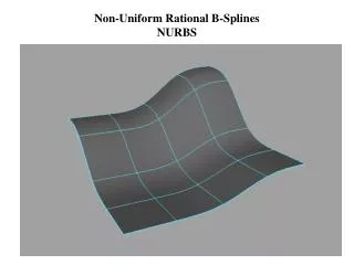
Non Uniform Rational B-Spline (NURBS)
270 likes | 693 Vues
Non Uniform Rational B-Spline (NURBS). NURBS. n. P(u) = w i N i,k (u)p i w i N i,k (u) NURBS curve degree = k-1 P 0 , P 1 ,..P n – control points Knot vector u = (u 0 , u 1 …u m ) W= (w 0 , w 1 …w m ) – weight non negative

Non Uniform Rational B-Spline (NURBS)
E N D
Presentation Transcript
Non Uniform Rational B-Spline (NURBS) disediakan oleh Suriati Bte Sadimon GMM, FSKSM, UTM, 2004
NURBS n • P(u) = wiNi,k(u)pi • wiNi,k(u) • NURBS curve degree = k-1 • P0, P1,..Pn – control points • Knot vector u = (u0, u1…um) • W= (w0, w1…wm) – weight non negative • The number of control points and the number of weights must agree • Use homogenous coordinates i=0 n i=0 disediakan oleh Suriati Bte Sadimon GMM, FSKSM, UTM, 2004
NURBS • If all wi are set to the value 1 or all wi have the same value we have the standard B-Spline curve • NURBS curve equation is a general form that can represent both B-Spline and NURBS curves. A Bezier curve is a special case of a B-Spline curve, so the NURBS equation can also represent Bezier and rational Bezier curves. disediakan oleh Suriati Bte Sadimon GMM, FSKSM, UTM, 2004
NURBS :important properties • NURBS have all properties of B-Spline.(pls refer to the notes) • Extra properties • More versatile modification of a curve becomes possible if the curve is represented by a NURBS equation. It is due to B-spline curve is modified by changing the x, y, z coord, but NURBS curve use homogenous coord (x, y, z, h) Or B-Spline (degree, control points & knots) but NURBS (degree, control points, knots & weights) disediakan oleh Suriati Bte Sadimon GMM, FSKSM, UTM, 2004
NURBS :important properties • Extra properties (cont) • NURBS equations can exactly represent the conic curves (circles, ellipse, parabola…) • Projective invariance If a projective transformation is applied to a NURBS curve, the result can be constructed from the projective images of its control points. Therefore, we do not have to transform the curve. We can obtain the correct view (no distortion). • * Bézier curves and B-spline curves only satisfy the affine invariance property rather than this projective invariance property. This is because only NURBS curves involve projective transformations. disediakan oleh Suriati Bte Sadimon GMM, FSKSM, UTM, 2004
NURBS : modifying weights • increasing the value of wi will pull the curve toward control point Pi. In fact, all affected points on the curve will also be pulled in the direction to Pi • When wi approaches infinity, the curve will pass through control point Pi • decreasing the value of wi will push the curve away from control point Pi disediakan oleh Suriati Bte Sadimon GMM, FSKSM, UTM, 2004
NURBS : modifying weights disediakan oleh Suriati Bte Sadimon GMM, FSKSM, UTM, 2004
NURBS : circle • NURBS equations represents the circle • Consider a half circle • Split the half circle into two circular arcs -1 and 2 (actually many ways) P2 P1 P3 2 1 P4 P0 disediakan oleh Suriati Bte Sadimon GMM, FSKSM, UTM, 2004
NURBS : circle • Consider arc 1 • Conic section (quadratic) – degree = 2 • 3 control points, P0= (1,0) ,P1 =(1,1), P2 = (0,1) • Knot value (0,0,0,1,1,1) • Weights w0 =1 w1 = cos = cos 45 = 1/2 w2=1 P2 P1 1 P0 disediakan oleh Suriati Bte Sadimon GMM, FSKSM, UTM, 2004
NURBS : circle • Follow the same procedure for arc 2 • We obtain • P2= (0,1) ,P3 =(-1,1), P4 = (-1,0) • Weights w2 =1, w3 = cos 45 = 1/2, w4=1 • Knot value =(0, 0, 0,1,1,1) shifted to (1, 1, 1, 2, 2, 2) for the composition P2 P3 2 P4 disediakan oleh Suriati Bte Sadimon GMM, FSKSM, UTM, 2004
NURBS : circle • Composite curve (arc 1 and arc 2) • P0= (1,0) ,P1 =(1,1), P2 = (0,1),P3 =(-1,1), P4 = (-1,0) • Weights w0 =1 w1 = 1/2 w2=1, w3 = 1/2, w4=1 • k = 3, n= 4 number of knot = 8 • Knot value =(0, 0, 0,1,1,1) + (1, 1, 1, 2, 2, 2) • Knot value = (0, 0, 0, 1, 1, 1, 2, 2, 2) shift 1 value • (0, 0, 0,1, 1, 2, 2, 2) P2 P1 P3 2 1 P4 P0 disediakan oleh Suriati Bte Sadimon GMM, FSKSM, UTM, 2004
NURBS : circle P2 • So, for a circle • P0= P8= (1,0) ,P1 =(1,1), P2 = (0,1),P3 =(-1,1), P4 = (-1,0), P5 =(-1,-1), P6 =(0,-1), P7 =(1,-1) • Weights w0 =1 w1 = 1/2 w2=1, w3 = 1/2, w4=1 • k = 3, n= 8 number of knot = 12 • (0, 0, 0,1, 1, 2, 2, 3, 3, 4, 4, 4) P1 P3 2 1 P4 P8 P0 P5 P7 P6 disediakan oleh Suriati Bte Sadimon GMM, FSKSM, UTM, 2004
NURBS : circle • Other way split into 3 arcs = 60 P3 P2 P4 P1 P5 P0 disediakan oleh Suriati Bte Sadimon GMM, FSKSM, UTM, 2004
NURBS : circle • show that NURBS equations exactly represent the circle • Consider arc 1 • NURBS equation is • P(u) = wiNi,k(u)pi • wiNi,k(u) • P(u) = w0P0N0, 3(u) + w1P1N1, 3(u) + w2P2N2, 3(u) • w0N0, 3(u) + w1N1, 3(u) + w2N2, 3(u) disediakan oleh Suriati Bte Sadimon GMM, FSKSM, UTM, 2004
NURBS : circle • w0 = w2 =1, w1 = 2 /2 • N0, 3= (1-u) 2, N1, 3= 2u(1-u), N2, 3= u2 pls refer to last topic (Curve1.pdf, slide 30) • P(u) = P0 (1-u) 2 +2 /2[P1 2u(1-u)]+ P2 u2 • (1-u) 2 +2 /2[2u(1-u)]+ u2 • P0 = [1,0,1] P1 = [1,1,1], P2 = [0,1,1] homogenous • x(u) = (1- 2) u2 +2 (1-2)u + 1 • (2- 2) u2 +(2-2)u + 1 • y(u) = ( 1- 2) u2 +2u . • (2- 2) u2 +(2-2)u + 1 • x(u) 2 + y(u) 2 = 1 - circle radius 1 prove!! disediakan oleh Suriati Bte Sadimon GMM, FSKSM, UTM, 2004
Knot Insertion : NURBS • three steps: (1) converting the given NURBS curve in 3D to a B-spline curve in 4D (2) performing knot insertion to this four dimensional B-spline curve (3) projecting the new set of control points back to 3D to form the the new set of control points for the given NURBS curve. disediakan oleh Suriati Bte Sadimon GMM, FSKSM, UTM, 2004
Knot Insertion : NURBS • EXAMPLE • a NURBS curve of degree 3 with a knot vector as follows: • 5 control points in the xy-plane and weights: • Insert new knot t = 0.4 disediakan oleh Suriati Bte Sadimon GMM, FSKSM, UTM, 2004
Knot Insertion : NURBS • t= 0.4 lies in knot span [u3 ,u4) • the affected control points are P3, P2, P1 and P0. • 1) convert to 3D B-Spline (homogenous coord) multiply all control points with their corresponding weights disediakan oleh Suriati Bte Sadimon GMM, FSKSM, UTM, 2004
Knot Insertion : NURBS 2) Perform knot insertion • compute a3, a2 and a1 a3 = t - u3 = 0.4 –0 = 0.4 u6 -u3 1 – 0 a2 = t - u2 = 0.4 –0 = 0.4 u5 -u2 1 – 0 a1 = t – u1 = 0.4 –0 = 0.8 u4 -u10.5 – 0 disediakan oleh Suriati Bte Sadimon GMM, FSKSM, UTM, 2004
Knot Insertion : NURBS • 2) Perform knot insertion (cont) • The new control points Qw3, Qw2 and Qw1 are: • Qw3 = (1-a3)Pw2+ a3Pw3 = (325.6, 26, 4.4) • Qw2 = (1-a2)Pw1+ a2Pw2 = (97.4, 142.5, 1.9) • Qw1 = (1-a1)Pw0+ a1Pw1 = (-42, 14.8, 0.6) disediakan oleh Suriati Bte Sadimon GMM, FSKSM, UTM, 2004
Knot Insertion : NURBS • 3) Projecting these control points back to 2D by dividing the first two components with the third (the weight), • Q3 = (74, 5.9 ) with weight 4.4 • Q2 = (51.3, 75 ) with weight 1.9 • Q1 = (-70, 24.6) with weight 0.6 disediakan oleh Suriati Bte Sadimon GMM, FSKSM, UTM, 2004
Knot Insertion : NURBS *control points in the xy-plane and weights after knot insertion *new knot vector disediakan oleh Suriati Bte Sadimon GMM, FSKSM, UTM, 2004