Grid Systems and scheduling
650 likes | 912 Vues
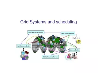
Grid Systems and scheduling. Grid systems. Many!!! Classification : (depends on the author) Computational grid : distributed supercomputing (parallel application execution on multiple machines) high throughput (stream of jobs)

Grid Systems and scheduling
E N D
Presentation Transcript
Grid systems • Many!!! • Classification: (depends on the author) • Computational grid: • distributed supercomputing (parallel application execution on multiple machines) • high throughput (stream of jobs) • Data grid:provides the way to solve large scale data management problems • Service grid:systems that provide services that are not provided by any single local machine. • on demand: aggregate resources to enable new services • Collaborative: connect users and applications via a virtual workspace • Multimedia: infrastructure for real-time multimedia applications
Taxonomy of Applications • Distributed supercomputingconsume CPU cycles and memory • High-Throughput Computingunused processor cycles • On-Demand Computingmeet short-term requirements for resources that cannot be cost-effectively or conveniently located locally. • Data-Intensive Computing • Collaborative Computingenabling and enhancing human-to-human interactions (eg: CAVE5D system supports remote, collaborative exploration of large geophysical data sets and the models that generated them)
Alternative classification • independent tasks • loosely-coupled tasks • tightly-coupled tasks
Application partitioning mapping allocation management grid node A grid node B Application Management • Description • Partitioning • Mapping • Allocation
Description • Use a grid application description language • Grid-ADL and GEL • One can take advantage of loop construct to use compilation mechanisms for vectorization
Grid-ADL Traditional systems 1 2 5 6 alternative systems 1 .. 2 5 6
Partitioning/Clustering • Application represented as a graph • Nodes: job • Edges: precedence • Graph partitioning techniques: • Minimize communication • Increase throughput or speedup • Need good heuristics • Clustering
Graph Partitioning • Optimally allocating the components of a distributed program over several machines • Communication between machines is assumed to be the major factor in application performance • NP-hard for case of 3 or more terminals
Collapse the graph • Given G = {N, E, M} • N is the set of Nodes • E is the set of Edges • M is the set of machine nodes
Dominant Edge • Take node nand its heaviest edge e • Edges e1,e2,…er with opposite end nodes not in M • Edges e’1,e’2,…e’k with opposite end nodes in M • If w(e) ≥ Sum(w(ei)) + max(w(e’1),…,w(e’k)) • Then the min-cut does not contain e • Soecan be collapsed
Machine Cut • Let machine cut Mi be the set of all edges between a machine miand non-machine nodes N • Let Wi be the sum of the weights of all edges in the machine cut Mi • Wi’s are sorted so W1 ≥ W2 ≥ … • Any edge that has a weight greater than W2 cannot be part of the min-cut
Zeroing • Assume that node n has edges to each of the m machines in M with weights w1 ≤ w2 ≤ … ≤ wm • Reducing the weights of each of the m edges from n to machines M by w1 doesn’t change the assignment of nodes for the min-cut • It reduces the cost of the minimum cut by (m-1)w1
Order of Application • If the previous 3 techniques are repeatedly applied on a graph until none of them are applicable: • Then the resulting reduced graph is independent of the order of application of the techniques
Output • List of nodes collapsed into each of the machine nodes • Weight of edges connecting the machine nodes • Source: Graph Cutting Algorithms for Distributed Applications Partitioning, Karin Hogstedt, Doug Kimelman, VT Rajan, Tova Roth, and Mark Wegman, 2001 • homepages.cae.wisc.edu/~ece556/fall2002/PROJECT/distributed_applications.ppt
Graph partitioning • Hendrickson and Kolda, 2000: edge cuts: • are not proportional to the total communication volume • try to (approximately) minimize the total volume but not the total number of messages • do not minimize the maximum volume and/or number of messages handled by any single processor • do not consider distance between processors (number of switches the message passes through, for example) • undirected graph model can only express symmetric data dependencies.
Graph partitioning • To avoid message contention and improve the overall throughput of the message traffic, it is preferable to have communication restricted to processors which are near to each other • But, edge-cut is appropriate to applications whose graph has locality and few neighbors
Resource Management (1988) Source: P. K. V. Mangan, Ph.D. Thesis, 2006
Static scheduling task precedence graphDSC: Dominance Sequence Clustering • Yang and Gerasoulis, 1994: two step method for scheduling with communication:(focus on the critical path) • schedule an unbounded number of completely connected processors (cluster of tasks); • if the number of clusters is larger than the number of available processors, then merge the clusters until it gets the number of real processors, considering the network topology (merging step).
Kwok and Ahmad, 1999: multiprocessor scheduling taxonomyStatic Scheduling Algorithms for Allocating Directed Task Graphsto Multiprocessors
List Scheduling • make an ordered list of processes by assigning them some priorities • repeatedly execute the following two steps until a valid schedule is obtained: • Select from the list, the process with the highest priority for scheduling. • Select a resource to accommodate this process. • priorities are determined statically before the scheduling process begins. The first step chooses the process with the highest priority, the second step selects the best possible resource. • Some known list scheduling strategies: • Highest Level First algorithm or HLF • Longest Path algorithm or LP • Longest Processing Time • Critical Path Method • List scheduling algorithms only produce good results for coarse-grained applications
Graph partitioning • Kumar and Biswas, 2002: MiniMax • multilevel graph partitioning scheme • Grid-aware • consider two weighted undirected graphs: • a work-load graph (to model the problem domain) • a system graph (to model the heterogeneous system)
Resource Management • The scheduling algorithm has four components: • transfer policy: whena node can take part of a task transfer; • selection policy: which taskmust be transferred; • location policy: which nodeto transfer to; • information policy: when to collectsystem state information.
Resource Management • Location policy: • Sender-initiated • Receiver-initiated • Symmetrically-initiated
Scheduling mechanisms for grid • Berman, 1998 (ext. by Kayser, 2006): • Job scheduler • Resource scheduler • Application scheduler • Meta-scheduler
Scheduling mechanisms for grid • Legion • University of Virginia (Grimshaw, 1993) • Supercomputing 1997 • Currently Avaki commercial product
Legion • is an object oriented infrastructure for grid environments layered on top of existing software services. • uses the existing operating systems, resource management tools, and security mechanisms at host sites to implement higher level system-wide services • design is based on a set of core objects
Legion • resource management is a negotiation between resources and active objects that represent the distributed application • three steps to allocate resources for a task: • Decision: considers task’s characteristics and requirements, resource’s properties and policies, and users’ preferences • Enactment: the class object receives an activation request; if the placement is acceptable, start the task • Monitoring: ensures that the task is operating correctly
Globus • Toolkit with a set of components that implement basic services: • Security • resource location • resource management • data management • resource reservation • Communication
Globus • From version 1.0 in 1998 to the 2.0 release in 2002 and the latest 3.0, the emphasis is to provide a set of components that can be used either independently or together to develop applications • The Globus Toolkit version 2 (GT2) design is highly related to the architecture proposed by Foster et al. • The Globus Toolkit version 3 (GT3) design is based on grid services, which are quite similar to web services. GT3 implements the Open Grid Service Infrastructure (OGSI). • The current version, GT4, is also based on grid services, but with some changes in the standard
Globus: scheduling • GRAM: Globus Resource Allocation Manager • Each GRAM responsible for a set of resources operating under the same site-specific allocation policy, often implemented by a local resource management • GRAM provides an abstraction for remote process queuing and execution with several powerful features such as strong security and file transfer • It does not provide scheduling or resource brokering capabilities but it can be used to start programs on remote resources, despite local heterogeneity due to the standard API and protocol.
Globus: scheduling • Resource Specification Language (RSL) is used to communicate requirements. • To take advantage of GRAM, a user still needs a system that can remember what jobs have been submitted, where they are, and what they are doing. • To track large numbers of jobs, the user needs queuing, prioritization, logging, and accounting. These services cannot be found in GRAM alone, but are provided by systems such as Condor-G
MyGrid and OurGrid • Mainly for bag-of-tasks (BoT) applications • uses the dynamic algorithm Work Queue with Replication (WQR) • hosts that finished their tasks are assigned to execute replicas of tasks that are still running. • Tasks are replicated until a predefined maximum number of replicas is achieved (in MyGrid, the default is one).
OurGrid • An extension of MyGrid • resource sharing system based on peer-to-peer technology • resources are shared according to a “network of favors model”, in which each peer prioritizes those who have credit in their past history of interactions.
GrADS • is an application scheduler • The user invokes the Grid Routine component to execute an application • The Grid Routine invokes the component Resource Selector • The Resource Selector accesses the Globus MetaDirectory Service (MDS) to get a list of machines that are alive and then contact the Network Weather Service (NWS) to get system information for the machines.
GrADS • The Grid Routine then invokes a component called Performance Modeler with the problem parameters, machines and machine information. • The Performance Modeler builds the final list of machines and sends it to the Contract Developer for approval. • The Grid Routine then passes the problem, its parameters, and the final list of machines to the Application Launcher.
GrADS • The Application Launcher spawns the job using the Globus management mechanism (GRAM) and also spawns the Contract Monitor. • The Contract Monitor monitors the application, displays the actual and predicted times, and can report contract violations to a re-scheduler.
GrADS • Although the execution model is efficient from the application perspective, it does not take into account the existence of other applications in the system
GrADS • Vadhiyar and Dongarra, 2002: proposed a metascheduling architecture in the context of the GrADS Project. • The metascheduler receives candidate schedules of different application level schedulers and implements scheduling policies for balancing the interests of different applications.
EasyGrid • Mainly concerned with MPI applications • Allows intercluster execution of MPI processes
Nimrod • uses a simple declarative parametric modeling language to express parametric experiments • provides machinery that automates task of: • formulating, • running, • monitoring, • collating results from the multiple individual experiments. • incorporates distributed scheduling that can manage the scheduling of individual experiments to idle computers in a local area network • has been applied to a range of application areas, e.g.: Bioinformatics, Operations Research, Network Simulation, Electronic CAD, Ecological Modelling and Business Process Simulation.
AppLeS • UCSD (Berman and Casanova) • Application parameter Sweep Template • Use scheduling based on min-min, min-max, sufferage, with heuristics to estimate performance of resources and tasks • Performance information dependent algorithms (pida) • Main goal: to minimize file transfers
Main scheduling algorithm sched() { (1) compute the next scheduling event (2) create a Gantt Chart, G (3) foreach computation and file transfer currently underway compute an estimate of its completion time fill in the corresponding blocks in G (4) until each host has been assigned enough work heuristically assign tasks to hosts (filling blocks in G) (5) convert G into a plan } Min-min, min-max, sufferage: step (4)
Min-min algorithm • A task list is generated that includes all the tasks as unmapped tasks. • For each task in the task list, the machine that gives the task its minimum completion time (first Min) is determined (ignoring other unmapped tasks). • Among all task-machine pairs found in 2, the pair that has the minimum completion time (second Min) is determined. • The task selected in 3 is removed from the task list and is mapped to the paired machine. • The ready time of the machine on which the task is mapped is updated. • Steps 2-5 are repeated until all tasks have been mapped. Source: Study of an Iterative Technique to Minimize Completion Times of Non-Makespan Machines, by Luis Diego Briceño, Mohana Oltikar, Howard Jay Siegel, and Anthony A. Maciejewski, 2007
Sufferage algorithm • A task list (L) is generated that includes all unmapped tasks in a given arbitrary order. • While there are still unmapped tasks: • Mark all machines as unassigned. • For each task tk є L. • The machine mjthat gives the earliest completion time is found. • The Sufferage value is calculated. (Sufferage value = second earliest completion time minus earliest completion time). • If machine mjis unassigned then assign tkto machine mj, delete tkfrom L, and mark mjas assigned. Otherwise, if the sufferage value of the task (ti) already assigned to mjis less than the sufferage value of task tkthen unassign ti, add tiback to L, assign tkto machine mj, and remove tkfrom L. • The ready times for all machines are updated. Source:Study of an Iterative Technique to Minimize Completion Times of Non-Makespan Machines, by Luis Diego Briceño, Mohana Oltikar, Howard Jay Siegel, and Anthony A. Maciejewski, 2007
Minimum Completion Time (MCT) algorithm • A task list is generated that includes all unmapped tasks in a given arbitrary order. • The first task in the list is mapped to its minimum completion time machine (machine ready time plus estimated computation time of the task on that machine). • The task selected in step 2 is removed from the task list. • The ready time of the machine on which the task is mapped is updated. • Steps 2-4 are repeated until all the tasks have been mapped. Source:Study of an Iterative Technique to Minimize Completion Times of Non-Makespan Machines, by Luis Diego Briceño, Mohana Oltikar, Howard Jay Siegel, and Anthony A. Maciejewski, 2007
GRAnD [Kayser et al., CCP&E, 2007] • Distributed submission control • Data locality • automatic staging of data • optimization of file transfer
Distributed submission Results of simulation with Monarc: http://monarc.web.cern.ch/MONARC/ [Kayser, 2006]
GRAnD • Experiments with Globus • Discussion list: discuss@globus.org (05/02/2004) • Submission takes 2s per task • Place 200 tasks in the queue: ~6min • Maximum number of tasks: few hundreds • experiments in CERN (D. Foster et al. 2003) • 16s to submit a task • Saturation in the server: 3.8 tasks/minute