FUNCTIONAL DEPENDENCIES
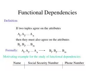
FUNCTIONAL DEPENDENCIES. Definition. Let R be the relation, and let x and y be the arbitrary subset of the set of attributes of R. Then we say that Y is functionally dependent on x – in symbol. X Y (Read x functionally determines y) –

FUNCTIONAL DEPENDENCIES
E N D
Presentation Transcript
Definition • Let R be the relation, and let x and y be the arbitrary subset of the set of attributes of R. Then we say that Y is functionally dependent on x – in symbol. X Y (Read x functionally determines y) – If and only if each x value in R has associated with it precisely one y value in R In other words Whenever two tuples of R agree on their x value, they also agree on their Y value. Deepak Gour, Faculty – DBMS, School of Engineering, SPSU
Example (SCP Relation) Deepak Gour, Faculty – DBMS, School of Engineering, SPSU
Example (SCP Relation) (contd..) One FD : - ( { S#} {City}) • Because every tuple of that relation with a given S# value also has the same city value. • The left and right hand side of an FD are sometimes called determinant and the dependents respectively. Deepak Gour, Faculty – DBMS, School of Engineering, SPSU
Exercise Check whether following relation satisfy FD as not • < S#, P# > <QTY> • <S#, P#> <City> • < S#, P#> <City, QTY> • <S#, P#> <S#> • <S#, P#> <S#, P#, QTY, City> • <OTY> <S#> Deepak Gour, Faculty – DBMS, School of Engineering, SPSU
Extended definition over basic one • Let R be the relation variable, and let x and y be arbitrary subset of the set of attributes of R. Then we says that Y is functionally dependent on x – in symbol. X Y (Read x functionally determines y) • If and only if, in every possible legal value of R, each x value has associated with it precisely one y value Or in other words • In every possible legal value of R, whenever two tuple agree on their X values, they also agree on their Y value. Deepak Gour, Faculty – DBMS, School of Engineering, SPSU
TRIVIAL & NON-TRIVIAL DEPENDENCIES • One-way to reduce the size of the set of FD we need to deal with is to eliminate the trivial dependencies. • An FD is trivial if and only if the right hand side is a subset of the left hand side. e.g. <S#, P#> <S#>. (Trivial) • Nontrivial dependencies are the one, which are not trivial. Deepak Gour, Faculty – DBMS, School of Engineering, SPSU
CLOSURE of a set of dependencies • The set of all FDs that are implied by a given set S of FDs is called the closure of S, denoted by S+ • So we need an algorithm which compute S+ from S. Deepak Gour, Faculty – DBMS, School of Engineering, SPSU
Algorithm CLOSURE (Z, S): = Z; DO “ forever” For each FD X -> Y in S Do; if X < CLOSURE [Z, S] /* <= “subset of” */ then CLOSURE [Z,S] : = CLOSURE [Z, Z] U Y; end; If CLOSURE [Z, S] did not change on this iteration. Then leave loop; /* Computation complete */ End; Deepak Gour, Faculty – DBMS, School of Engineering, SPSU
Example Suppose use are given R with attributes A, B, C, D, E, F, and FDs • A BC • E CF • B E • CD EF Then compute the closure (A, B)+ of the set of attributes under this set of FD’s Deepak Gour, Faculty – DBMS, School of Engineering, SPSU
Solution • We initialize the result CLOSURE [Z, S] to <A, B> • We now go round the inner loop four times, once for each for the given FDs. An the first iteration (For FD A BC), we find that the left hand side is indeed a subset of CLOSURE (Z, S) as computed so for, so we add attributes (B and C) to the result. CLOSURE [Z, S] is now the set <A, B, C>. Deepak Gour, Faculty – DBMS, School of Engineering, SPSU
Solution 3. On the second iteration (for FD E CF>. we find that the left hand side is not a subset of the result as computed so for, which than remain unchanged. • On the third iteration (For FD B E), we add E to the closure, which now has the value <A, B, C, E> • On the fourth iteration, (for FD CD EF), remains unchanged. Deepak Gour, Faculty – DBMS, School of Engineering, SPSU
Solution • Inner loop times, on the first iteration no change, second, it expands to <A,B, C, E, F> third & fourth, no change. • Again inner loop four times, no change, and so the whole process terminates. Deepak Gour, Faculty – DBMS, School of Engineering, SPSU
Armstrong rules • Reflexivity: if B is a subset of A, then A B. • Augmentation: if A B then AC BC • Transitivity: it A B and B C then A C. • Self – determination: A A. • Decomposition: If A BC, then AB, AC. • Union: it A B and A C, then A BC • Composition: if A B, C D then AC BD. • If A B and C D, then All (C – B) BD Deepak Gour, Faculty – DBMS, School of Engineering, SPSU
Armstrong rules (contd..) • Now we define a set of FD to be irreducible as minimal; if and only if it satisfies the following two properties. (1) The right hand side of every FD in S involve just one attribute (i.e., it is a singleton set) (2) The left hand side of every FD in S is irreducible in turn meaning that no attribute can be discarded from the determinant without changing the CLUSURE S+. Deepak Gour, Faculty – DBMS, School of Engineering, SPSU
Example • A BC, • B C • A B • AB C • AC D Compute an irreducible set of FD that is equivalent to this given set. Deepak Gour, Faculty – DBMS, School of Engineering, SPSU
Solution (1) The step is to rewrite the FD such that each has a singleton right hand side. • A B • A C • B C • A B • AB C • AC D We observe that the FD A B occurs twice. So one occurrence will be eliminated. Deepak Gour, Faculty – DBMS, School of Engineering, SPSU
Solution • Next, attributed C can be eliminated from the left hand side of the FD AC D • Because we have A C, • By augmentation A AC • And we are given AC D, • So A D by transitivity; Thus C on the left hand side is redundant. Deepak Gour, Faculty – DBMS, School of Engineering, SPSU
Solution 3. Next, we observe that the FD AB C can be eliminated, because again we have A C By augmentation AB CB By decomposition AB C 4. Finally, the FD A C is implied by the FD A B and B C, so it can be eliminated. Now we have A B B C A D This set is irreducible. Deepak Gour, Faculty – DBMS, School of Engineering, SPSU
Example • A BC • B E • CD EF Show that FD AD F for R. Deepak Gour, Faculty – DBMS, School of Engineering, SPSU
Solution 1. A BC (given) 2. A C (1, decomposition) 3. AD CD (2, augmentation) 4. CD EF (given) 5. AD EF (3 & 4, transitivity) 6. AD F (5, decomposition Deepak Gour, Faculty – DBMS, School of Engineering, SPSU
Learning Objectives • Definition of normalization and its purpose in database design • Types of normal forms 1NF, 2NF, 3NF, BCNF, and 4NF • Transformation from lower normal forms to higher normal forms • Design concurrent use of normalization and E-R modeling are to produce a good database design • Usefulness of denormalization to generate information efficiently Deepak Gour, Faculty – DBMS, School of Engineering, SPSU
Normalization • Main objective in developing a logical data model for relational database systems is to create an accurate representation of the data, its relationships, and constraints. • To achieve this objective, must identify a suitable set of relations. Deepak Gour, Faculty – DBMS, School of Engineering, SPSU
Normalization • Four most commonly used normal forms are first (1NF), second (2NF) and third (3NF) normal forms, and Boyce–Codd normal form (BCNF). • Based on functional dependencies among the attributes of a relation. • A relation can be normalized to a specific form to prevent possible occurrence of update anomalies. Deepak Gour, Faculty – DBMS, School of Engineering, SPSU
Normalization • Normalization is the process for assigning attributes to entities • Reduces data redundancies • Helps eliminate data anomalies • Produces controlled redundancies to link tables • Normalization stages • 1NF - First normal form • 2NF - Second normal form • 3NF - Third normal form • 4NF - Fourth normal form Deepak Gour, Faculty – DBMS, School of Engineering, SPSU
Data Redundancy • Major aim of relational database design is to group attributes into relations to minimize data redundancy and reduce file storage space required by base relations. • Problems associated with data redundancy are illustrated by comparing the following Staff and Branch relations with the StaffBranch relation. Deepak Gour, Faculty – DBMS, School of Engineering, SPSU
Data Redundancy Deepak Gour, Faculty – DBMS, School of Engineering, SPSU
Data Redundancy • StaffBranch relation has redundant data: details of a branch are repeated for every member of staff. • In contrast, branch information appears only once for each branch in Branch relation and only branchNo is repeated in Staff relation, to represent where each member of staff works. Deepak Gour, Faculty – DBMS, School of Engineering, SPSU
Update Anomalies • Relations that contain redundant information may potentially suffer from update anomalies. • Types of update anomalies include: • Insertion, • Deletion, • Modification. Deepak Gour, Faculty – DBMS, School of Engineering, SPSU
Functional Dependency • Main concept associated with normalization. • Functional Dependency • Describes relationship between attributes in a relation. • If A and B are attributes of relation R, B is functionally dependent on A (denoted A B), if each value of A in R is associated with exactly one value of B in R. Deepak Gour, Faculty – DBMS, School of Engineering, SPSU
Functional Dependency • Property of the meaning (or semantics) of the attributes in a relation. • Diagrammatic representation: • Determinant of a functional dependency refers to attribute or group of attributes on left-hand side of the arrow. Deepak Gour, Faculty – DBMS, School of Engineering, SPSU
Example - Functional Dependency Deepak Gour, Faculty – DBMS, School of Engineering, SPSU
Functional Dependency • Main characteristics of functional dependencies used in normalization: • have a 1:1 relationship between attribute(s) on left and right-hand side of a dependency; • hold for all time; • are nontrivial. Deepak Gour, Faculty – DBMS, School of Engineering, SPSU
Functional Dependency • Complete set of functional dependencies for a given relation can be very large. • Important to find an approach that can reduce set to a manageable size. • Need to identify set of functional dependencies (X) for a relation that is smaller than complete set of functional dependencies (Y) for that relation and has property that every functional dependency in Y is implied by functional dependencies in X. Deepak Gour, Faculty – DBMS, School of Engineering, SPSU
The Process of Normalization • Formal technique for analyzing a relation based on its primary key and functional dependencies between its attributes. • Often executed as a series of steps. Each step corresponds to a specific normal form, which has known properties. • As normalization proceeds, relations become progressively more restricted (stronger) in format and also less vulnerable to update anomalies. Deepak Gour, Faculty – DBMS, School of Engineering, SPSU
Relationship Between Normal Forms Deepak Gour, Faculty – DBMS, School of Engineering, SPSU
Unnormalized Form (UNF) • A table that contains one or more repeating groups. • To create an unnormalized table: • transform data from information source (e.g. form) into table format with columns and rows. Deepak Gour, Faculty – DBMS, School of Engineering, SPSU
First Normal Form (1NF) • A relation in which intersection of each row and column contains one and only one value. Deepak Gour, Faculty – DBMS, School of Engineering, SPSU
UNF to 1NF • Nominate an attribute or group of attributes to act as the key for the unnormalized table. • Identify repeating group(s) in unnormalized table which repeats for the key attribute(s). Deepak Gour, Faculty – DBMS, School of Engineering, SPSU
UNF to 1NF • All key attributes defined • No repeating groups in table • All attributes dependent on primary key Deepak Gour, Faculty – DBMS, School of Engineering, SPSU
Second Normal Form (2NF) • Based on concept of full functional dependency: • A and B are attributes of a relation, • B is fully dependent on A if B is functionally dependent on A but not on any proper subset of A. • 2NF - A relation that is in 1NF and every non-primary-key attribute is fully functionally dependent on the primary key (no partial dependency) Deepak Gour, Faculty – DBMS, School of Engineering, SPSU
1NF to 2NF • Identify primary key for the 1NF relation. • Identify functional dependencies in the relation. • If partial dependencies exist on the primary key remove them by placing them in a new relation along with copy of their determinant. Deepak Gour, Faculty – DBMS, School of Engineering, SPSU
2NF Conversion Results Figure 4.5 Deepak Gour, Faculty – DBMS, School of Engineering, SPSU
Third Normal Form (3NF) • Based on concept of transitive dependency: • A, B and C are attributes of a relation such that if A B and B C, • then C is transitively dependent on A through B. (Provided that A is not functionally dependent on B or C). • 3NF - A relation that is in 1NF and 2NF and in which no non-primary-key attribute is transitively dependent on the primary key. Deepak Gour, Faculty – DBMS, School of Engineering, SPSU
2NF to 3NF • Identify the primary key in the 2NF relation. • Identify functional dependencies in the relation. • If transitive dependencies exist on the primary key remove them by placing them in a new relation along with copy of their determinant. Deepak Gour, Faculty – DBMS, School of Engineering, SPSU
3NF Conversion Results • Prevent referential integrity violation by adding a JOB_CODE PROJECT (PROJ_NUM, PROJ_NAME) ASSIGN (PROJ_NUM, EMP_NUM, HOURS) EMPLOYEE (EMP_NUM, EMP_NAME, JOB_CLASS) JOB (JOB_CODE, JOB_DESCRIPTION, CHG_HOUR) Deepak Gour, Faculty – DBMS, School of Engineering, SPSU
General Definitions of 2NF and 3NF • Second normal form (2NF) • A relation that is in 1NF and every non-primary-key attribute is fully functionally dependent on anycandidate key. • Third normal form (3NF) • A relation that is in 1NF and 2NF and in which no non-primary-key attribute is transitively dependent on any candidate key. Deepak Gour, Faculty – DBMS, School of Engineering, SPSU
Boyce–Codd Normal Form (BCNF) • Based on functional dependencies that take into account all candidate keys in a relation, however BCNF also has additional constraints compared with general definition of 3NF. • BCNF - A relation is in BCNF if and only if every determinant is a candidate key. Deepak Gour, Faculty – DBMS, School of Engineering, SPSU
Boyce–Codd normal form (BCNF) • Difference between 3NF and BCNF is that for a functional dependency A B, 3NF allows this dependency in a relation if B is a primary-key attribute and A is not a candidate key. • Whereas, BCNF insists that for this dependency to remain in a relation, A must be a candidate key. • Every relation in BCNF is also in 3NF. However, relation in 3NF may not be in BCNF. Deepak Gour, Faculty – DBMS, School of Engineering, SPSU