Functional Dependencies

1. Functional Dependencies Jorge Pombar

2. Functional dependencies are the building blocks that enable the analysis of data redundancy and the elimination of anomalies caused by data redundancy through the process of normalization. Normalization is a technique that facilitates systematic validation of participation of attributes in a relation schema from a perspective of data redundancy. Definitions

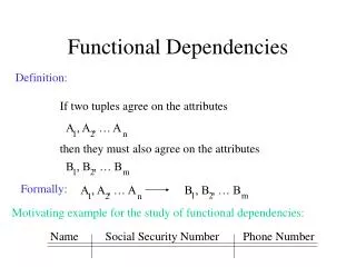
3. An attribute A in a relation schema R functionally determines another attribute B in R if for a given value a1 of A there is a single, specified value b1 of B in the relation r of R. A and B can be either atomic or composite. A symbolic representation of this: FD is: A->B In other words for A->B to be true. If two tuples in r(R) have the same A values then they must have the same B values. Functional Dependencies (FD)

4. Notation • A (the left-side of the FD) is the determinant and B (the right-side of the FD) is the dependant. • If the determinant or the dependant are composite values then the atomic values are enclosed in braces. {Store, Product} -> Quantity

5. Example • Stock table. Normalized or unnormalized? • Unnormalized! • Let’s take a closer look. • Is Quantityredundant? • How about Price? • What about Location and Discount?

6. Anomalies • Anomalies happen when a database operation produces the undesired result of affecting the integrity of the database. • Three types: • Insertion anomaly • Deletion anomaly • Update anomaly • The three anomalies combined are known as modification anomalies.

7. Example • We want to add a blender and its Price to our stock. We can’t unless we know the store where they’ll be stocked. • Insertion anomaly! • If we close store 17 we have to change multiple lines and we loose the info on the price of the vacuum cleaner. • Deletion anomaly! • If we want to change theLocation of store 11 we have to change all rows were store 11 appears. • Modification anomaly!

8. We “split” the data into separate tables to eliminate redundancies. How do we fix it? Inventory

9. New tables Store Product

10. New tables (cont.) • This new system is less efficient when retrieving data. That’s the price paid for eliminating the modification anomalies. • We draw the line between efficiency and redundancy. • Discount is stored redundantly. This is called controlled redundancy and is done for efficiency of data retrieval.

11. Inference rules for FDs • The set of functional dependencies explicitly specified on a relational schema is referred a F. • Given F it is possible to deduce all other FD’s in R that are not explicitly defined. • Closure is the set of all possible functional dependencies that hold in R. It is also referred as F+.

12. Armstrong’s Axioms • In 1974 William W. Armstrong proposed a systematic approach to derive all possible functional dependencies that can be inferred from F using what is now known as Armstrong Axioms.

13. Armstrong’s Axioms (cont.)

14. Armstrong’s Axioms (cont.) • Four more rules can be derived from the previous three.

15. Minimal Cover for a set of FDs • It is always useful to identify a simplified set of FDs, Gc, that is equivalent to F. This means that they have the same closure (F+) as F and its no further reducible. • We try to get the set G where F ≡ G. This means that we could enforce G or F and the valid database states will remain the same. • In practice the minimal cover is useful because the effort required to check for violations in the database is minimized therefore improving the database performance.

16. Minimal Cover for a set of FDs (cont.) • F can be its own minimal cover also known as canonical cover. • There can be several minimal covers of F. • Formally Gc is the minimal cover of F if: • Gc ≡ F • The dependant (RHS) in every FD in Gc is a singleton attribute. This is called standard or canonical form. • No FD in Gc is redundant. In other words, if any FD in Gc is discarded, then Gc would be no longer equivalent to F. • The determinant (LHS) if every FD in Gc is irreducible. In other words, if any attribute is discarded from the determinant of any FD in Gc, then Gc would be no longer equivalent to F.

17. Algorithm to compute the minimal cover • Set G to F. • Convert all FDs into standard (canonical) form. • Remove all redundant attributes from the determinant (LHS) of the FDs from G • Remove all redundant FDs from G. Two Notes: • This algorithm might produce different results based on the order of candidates removal. • Steps 3 and 4 aren’t interchangeable.

18. Examples • Consider a set of attributes {ABC} and set of FDs F: fd1: A->C fd2: (AC)->B fd3: B->A fd4: C->(AB) • Rewrite in standard form fd4: fd4a: C->A fd4b: C->B

19. Examples (cont.) • Based on fd4b, A in fd2 is redundant. We remove it. Now we remove fd4b because is identical to fd2. • We are left with the minimal cover of F (Gc): fd1: A->B fd2: B->C fd3: C->A

20. Examples (cont.) • Consider the set of attributes {Student,Advisor,Subject,Grade} and a set of FDs F: fd1:{Student,Advisor}->{Grade,Subject} fd2: Advisor->Subject fd3: {Student, Subject}->{Grade,Advisor} • Rewrite in standard form: fd1a: {Student,Advisor}->Grade fd1b: {Student,Advisor}->Subject fd2: Advisor->Subject fd3a: {Student,Subject}->Grade fd3b: {{Student,Subject}->Advisor

21. Examples (cont.) • Given fd2, Student is redundant in fd1b. We remove it. Now we remove fd1b since its identical to fd2. • Next, fd1a is redundant because it’s contained by the set {fd2, fd3a}. We remove it. • We are left with the minimal cover of F (Gc): fd2:Advisor->Subject fd3a: {Student,Subject}->Grade fd3b: {Student,Subject}->Advisor

22. Conclusion • After we have the ER diagrams each relation in the schema must be independently reviewed and normalized when needed. • This process gives us the final opportunity to correct errors and establish a robust design before implementing the database system.

23. References Lotito, J. (2001). Concepts of Database Design and Management. Retrived September 2007 from http://www.sitepoint.com/article/database-design-management Scamell, R.W., & Umanath N.S. (2007). Data Modeling and Database Design: Boston, MA: Thomson.