Download
1 / 33
360 likes | 1.1k Vues
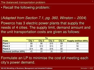
The Transportation Problem. ARE 511. Usually, we have a given capacity of goods at each source and a given requirement for the goods at each destination.

E N D
The Transportation Problem ARE 511
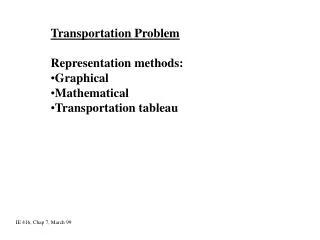
Usually, we have a given capacity of goods at each source and a given requirement for the goods at each destination. The objective of such a transportation problem is to schedule shipments from sources to destinations so that total transportation costs are minimized. Although LP can be used to solve this type of problem, more efficient special-purpose algorithms have been developed for the transportation application. As in the simplex algorithm, they involve finding an initial feasible solution and then making step-by-step improvements until an optimal solution is reached.
Unlike the simplex method, the transportation methods are fairly simple in terms of computation. To begin the analysis of a transportation problem, management must determine time costs of shipping from each source to each destination. Such data are usually presented in tabular form, as seen in the Table for the ease of the Executive Furniture Corp., a manufacturer of office desks. The next step is the setting up of a transportation table; its purpose is to summarize all relevant data concisely and to keep track of algorithm computations. We now construct a transportation table and label its various components.
DEVELOPING AN INITIAL SOLUTION— THE NORTHWEST CORNER RULE • Once the data have been arranged in tabular form, we must establish an initial feasible solution to the problem (just as we did in the first LP simplex table). • One systematic procedure, known as the northwest corner rule, requires that we start in the upper left hand cell (or northwest corner) of the table and allocate units to shipping routes as follows: • Exhaust the supply ( factory supply) at each row before moving down to the next row. • Exhaust the (warehouse) requirements of each column before moving to the next column, on the right. • Check that all the supply and demands are met.
EXAMPLE 13.1 • We can use the northwest corner rule to find an initial feasible solution to the Executive Furniture Corp. problem shown in the Table. • It takes five steps in this example to make the initial shopping assignments: • Assign 100 units from Des Moines to Albuquerque (exhausting Des Moines supply). • Assign 200 units from Evansville to Albuquerque (exhausting Albuquerque’s demand). • Assign 100 units from Evansville to Boston (exhausting Evansville’s supply). • Assign 100 units from Ft. Lauderdale to Boston (exhausting Boston’s demand). • Assign 200 units from Ft. Lauderdale to Cleveland (exhausting Cleveland’s demand and Ft. Lauderdale’s supply).
The solution given here is feasible since demand-and-supply constraints are all satisfied. It would be very lucky if this solution yielded the minimal transportation cost for the problem, however. It is more likely that one of the iterative procedures designed to help reach an optimal solution shall have to be employed. First, try to use the method to solve Problem 13.1.
The Stepping-Stone Method The stepping-stone method is an iterative technique for moving from an initial feasible solution to an optimal solution. It is used to evaluate the cost effectiveness of shipping goods via transportation routes not currently in the solution. Each unused cell, or square, in the transportation table is tested by asking the following question:What would happen to total shipping costs if one unit of product (for example, one desk) were tentatively shipped on an unused route ?
This testing of each unused square is conducted as follows: • Select an unused square to be evaluated. • Beginning at this square, trace a closed path back to the original square via squares that are currently being used (only horizontal and vertical moves are allowed). • Beginning with a plus (+) sign at the unused square, place alternate minus (-) signs and plus signs on each corner square of time closed path just traced. • Calculate an “improvement index” by adding together the unit cost figures found in each square containing a plus sign and then subtracting the unit costs in each square containing a minus sign. • Repeat steps l – 4 until an improvement index has been calculated for all unused squares. If all indices computed are greater than or equal to zero, an optimal solution lies been reached. If not, it is possible to improve the current solution and decrease total shipping costs
EXAMPLE 13.2 The stepping-stone method can be applied to the Executive Furniture Corp. data in Example 13.1 to evaluate unused shipping routes. The four currently used routes are seen to be: Des Moines to Boston, Des Moines to Cleveland, Evansville to Cleveland and Fort Lauderdale to Albuquerque. Beginning with the Des Moines to Boston route we first trace a closed path using only currently occupied squares (see the table), and then place alternate plus signs and minus signs in the corners of this path. To indicate more clearly the meaning of a closed path, we see that only squares currently used for shipping can be used in turning the corners of the route being traced.
Hence, the path Des Moines - Boston to Des Moines - Albuquerque to Fort Lauderdale - Albuquerque to Fort Lauderdale - Boston to Des Moines - Boston would not be acceptable since the Fort Lauderdale - Albuquerque square is currently empty. It can be seen that only one closed route is possible for each square that we wish to test . How to decide which squares are given plus signs and which minus signs? The answer: Since we are testing the cost effectiveness of the Des Moines to Boston shipping route, we pretend we are shipping one desk from Des Moines to Boston. This is one more unit that we are sending between the two cities, so we place a plus sign in the box. But, if we ship one more unit than before from Des Moines to Boston, we end up sending 101 desks out of the Des Moines factory.
That factory’s capacity is only 100 units, hence we must ship one desk less from Des Moines to Albuquerque, - this change made to avoid violating the limit constraint. To indicate that the Des Moines to Albuquerque shipment has been reduced, we place a minus sign in its box. Continuing along the closed path, we notice that we are no longer meeting the warehouse requirements of 300 units. In fact, if the Des Moines to Albuquerque shipment is reduced to 99 units the Evansville to Albuquerque load has to be increased by one unit, to 201 desks. Therefore, we place a plus sign in that box to indicate the increase. Finally, we note that if the Evansville to Albuquerque route is assigned 201 desks, the Evansville to Boston route must be reduced by one unit, to 99 desks, in order to maintain the Evansville factory capacity constraint of 300 units.
Thus, a minus sign is placed in the Evansville to Boston box. We observe below that all four routes on the closed path are hereby balanced in terms of demand- supply limitations. An improvement index for the Des Moines - Boston route is now computed by adding unit costs in squares with plus signs and subtracting costs in squares with minus signs. Hence Des Moines – Boston index = + $4 - $5 + $8 - $4 = +$3
This means that for every desk shipped via the Des Moines - Boston route, total transportation costs will increase by $3 over their current level. Let us now examine the Des Moines - Cleveland unused route, one slightly more difficult to trace with a closed path. Again, you will notice that we turn each corner along the path only at squares which represent existing routes. The path can go through the Evansville – Cleveland box but cannot turn a corner or place a or - sign there. Only an occupied square may be used as a “stepping stone”
Des Moines – Cleveland index = +$3 - $5 + $8 - $4 + $7 - $5 = $4 Thus, opening this route will also not lower our total shipping costs. The other two routes may be evaluated in a similar fashion. Evansville – Cleveland index = +$3 - $4 + $7 - $5 = +$1 (Closed path is +EC – EB + FB – FC) Fort Lauderdale – Albuquerque index = +$9 - $7 + $4 - $8 = -$2 (Closed path is +FA – FB + EB – EA) Because the second index is negative, a cost savings may be attained by making use of the (currently unused) Fort Lauderdale to Albuquerque route.
We saw, in Example 13.2 that a better solution is possible - this due to the presence of a negative improvement index on one of the unused routes. Each negative index represents the amount by which total transportation costs could be decreased if one unit or product were shipped by that source—destination combination. The next step, then, is to choose that route (unused square) with the largest negative improvement index. We can then ship the maximum allowable number of units on that route and reduce the total cost accordingly. The maximum quantity that can be shipped on the new money-saving route can be found by referring to the closed path of plus signs and minus signs drawn for the route and selecting the smallest number found in those squares containing minus signs.
To obtain a new solution, that number is added to all squares on the closed path with plus signs and subtracted from all squares on the path assigned minus signs. One iteration of the stepping-stone method is now complete. Again, we must test to see if it is optimal or whether any further improvements can be made. That is done by evaluating each unused square as described in the steps listed earlier.
EXAMPLE 13.3 To improve Executive Furniture’s solution we make use of the improvement indices calculated in Example 13.2. The largest (and only) negative index is found on the Fort Lauderdale to Albuquerque route. We repeat the transportation table for the problem below The maximum quantity that may be shipped on the newly opened route (FA) is the smallest number found in squares containing minus signs—-in this case, 100 units.
Hence, we add 100 units to the 0 now being shipped on route FA; then proceed to subtract 100 from route FB, leaving zero in that square (but still balancing the row total for F); then add 100 to route B yielding 200; and finally, subtract 100 from route EA, leaving 100 units shipped. Note that the new members still produce the correct row and column totals as required. The new solution is shown in the following table:
Total shipping cost has been reduced by (100 units) X ($2 saved/unit) = 200,and is now $4,000, This cost figure can, of course, also be derived by multiplying each unit shipping cost times the number of units transported on its route, namely, lOO($5) + l00( $8) + 100($9) + 200($5) = $4,000
Demand Not Equal To Supply A situation occurring quite frequently in real-world problems is the case where total demand is not equal to total supply. These unbalanced problems can be handled easily by the solution procedures discussed above if we first in introduce dummy sources or dummy destinations. In the event that total supply is greater than total demand, a dummy destination, with demand exactly equal to the surplus, is created. If total demand is greater than total supply, we introduce a dummy source (factory) with a supply equal to the excess of demand over supply. In either ease, cost coefficients of zero are assigned to each dummy location.
EXAMPLE 13.4 Executive Furniture Increases the rate of production of desks in its Des Moines factory to 250. To reformulate this unbalanced problem, we refer back to the data presented in Example 13.1. The northwest corner rule is used to find the initial feasible solution below. New Des Moines Capacity total cost = (250)($5) + (50)($8) + (200)($4) + 50($3) + 150($5) + 150($0) = $3,350
Degeneracy In order for the stepping-stone method to be applied to a transportation problem, a rule pertaining to the number of shipping routes being used must be observed. That rule may be stated as follows: The number of occupied squares in any solution (initial or later) must be equal to the number of rows in the table plus the number of columns minus 1. When this rule is not met, the solution is called degenerate. Usually, degeneracy occurs when there are too few squares, or shipping routes, being used. When this happens, it becomes impossible to trace a closed path for each unused square.
You might observe that no problem discussed in this unit thus far has been degenerate. The original furniture problem, for example, had 5 assigned routes (= 3 rows or factories + 3 columns or warehouses - 1). Example 13.4, employing a dummy warehouse had 6 assigned routes ( = 3 rows + 4 columns - 1) and was also not degenerate. To handle degenerate problems, we artificially create an occupied cell that is, if we place a zero (representing a fake shipment) in one of the unused squares and then treat that square as it were occupied. This square chosen, it should be noted, must be in such a position as to allow all stepping-stone paths to be chosen.
EXAMPLE 13.5 Martin Shipping Co. has three warehouses from which to supply its three major retail customers in San Jose. Martin’s shipping costs, warehouse supplies, and customer demands are made in the following transportation table. Initial shipping assignments are made in the table by application of the northwest corner rule. This initial solution is degenerate because it violates the rule that the number of used squares be equal to the number of rows + the number of columns.
To correct the problem, we may place a 0 in the unused square representing the shipping route from warehouse 2 to customer 1. Now all stepping-stone paths can be closed and improvement indices computed.
The Modi Method The MODI (modified distribution) method allows us to compute indices for each unused square without drawing all the closed paths. Because of this, it can often provide considerable time savings over the stepping-stone method for solving transportation problems. In applying the MODI method, we begin with an initial solution obtained by using the northwest corner rule. But now, we must compute a value for each row (call the values R1, R2, R3 if there are 3 rows) and for each column (K1, K2, K3) in the transportation table.
In general, we let • Ri = value assigned to row i. • Kj = value assigned to column j. • Cij = cost in square ij (cost of shipping from source i to destination j). • The MODI method then requires three steps: • To compute the values for each row and column, set Ri + Kj = Cij but only for those squares that are currently used or occupied. • After all equations have been written, set R1 = 0. • Solve the system of equations for all R and K values. • Compute the improvement index for each unused square by the formula: Cij – Ri – Kj. • Select the largest negative index and proceed to solve the problem as we did using the stepping-stone method.
EXAMPLE 13.6 Given the initial solution to the Executive furniture problem (from Example 13.1), we can use the MODI method to calculate an improvement index for each unused square. The initial transportation table is repeated below.
We first set up an equation for each occupied square: • R1 + K1 = 5 • R2 + K1 = 8 • R2 + K2 = 4 • R3 + K2 = 7 • R3 + K3 = 5 • Letting R1 = 0, we can easily solve, step by step, for K1, R2, K2, R3 and K3. • 0 + K1 = 5 K1 = 5 • R2 + 5 = 8 R2 = 3 • 3 + K2 = 4 K2 = 1 • R3 + 1 = 7 R3 = 6 • 6 + K3 = 5 K3 = -1
The improvement index for each unused cell is Cij – Ri – Kj. • Des Moines to Boston = C12 – R1 – K2 = 4 – 0 – 1 = $3. • Des Moines to Cleveland = C13 – R1 – K3 = 3 – 0 – ( - 1) = $4. • Evansville to Cleveland = C23 – R2 – K3 = 3 – 3 – ( - 1) = $1. • Ft. Lauderdale to Albuquerque = C31 – R3 – K1 = 9 – 6 – 5 = - $2. • Note that these indices are exactly the same as the ones calculated in Example 13.2. It is now necessary to trace only one closed path, for Ft. Lauderdale to Albuquerque, in order to proceed with the solution procedures as used in the stepping-stone method.
Homework problems • Problem 13.1 – Northwest Corner Method • Problem 13.2 – Stepping-stone Method • Problem 13.3 – Stepping-stone Method • Problem 13.4 – Dummy Sources Method • Problem 13.5 – Degeneracy • Problem 13.1 – MODI Method