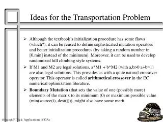
1. Ideas for the Transportation Problem • Although the textbook’s initialization procedure has some flaws (which?), it can be reused to define sophisticated mutation operators and better initialization procedures (by taking a random number in [0,min] instead of the minimum). Moreover, it can be used to develop randomized hill climbing style systems. • If M1 and M2 are legal solutions, a*M1 + b*M2 (with a,b>0 a+b=1) are also legal solutions. This provides as with a quite natural crossover operator. This operator is called arithmetical crossover in the EC numerical optimization literature. • Boundary Mutation (that sets the value of one (possibly more) elements of the matrix to its minimum (0) or maximum possible value (min(source(i), dest(j))), might also have some merit.

2. Some Initial Thoughts on the Course Project • Have a general theme • Compare at least 2 approaches (could be similar) • Run algorithms at least 3 times (you might just be unlucky) • Report the results of running the benchmark transparently and completely • Interpret your results (even if there is no clear evidence pointing into one direct); explain your results (could be speculative) • Report the history of the project • Be prepared to demo your program shortly after the due date. • What was expected, what was unexpected?

3. Conducting Experiments in General and in the Context of the Transportation Problem • Things to observe when running an EC-system • Average fitness • Best solution found so far • Diversity in the current population (expensive) • Degree of change from generation to generation • Visualizing the current best solutions could be helpful • Size of searched solutions; building blocks in the searched solutions • Complexity: runtime, storage, number of genetic operators applied,… • What parts of the search space are searched (hard to analyze) • Things to report when summarizing experiments • Experimental Environment: Operators used and probabilities of their application, selection method, population size, best found solution, best average fitness. • Observed Results: Best solution found, best fitness/average fitness over time, diversity over time.

4. Requirements for TSP-Crossover Operators • Edges that occur in both parents should not be lost. • Introducing new edges that do not occur in any parent should be avoided. • Producing offspring that are very similar to one of the parents but do not have any similarities with the other parent should be avoided. • It is desirable that the crossover operator is complete in the sense that all possible combinations of the features occuring in the two parents can be obtained by a single or a sequence of crossover operations. • The computational complexity of the crossover operator should be low. ER DR, TD

5. Donor-Receiver-Crossover (DR) 1) Take a path of significant length (e.g. between 1/4 and 1/2 of the chromosome length) from one parent called the donor; this path will be expanded by mostly receiving edges from the other parent, called the receiver. 2) Complete the selected donor path giving preference to higher priority completions: P1: add edges from the receiver at the end of the current path. P2: add edges from the receiver at the beginning of the current path. P3: add edges from the donor at the end of the current path. P4: add edges from the donor at the start of the current path. P5: add an edge including an unassigned city at the end of the path. • The basic idea for this class of operator has been introduced by Muehlenbein.

6. Top-Down Edge Preserving Crossovers (TD) 1) Take all edges that occur in both parents. 2) Take legal edges from one parent alternating between parents, as long as possible. 3) Add edges with cities that are still missing. • Michalewicz matrix crossover and many other crossover operators employ this scheme.

7. Typical TSP Mutation Operators • Inversion (like standard inversion): • Insertion (selects a city and inserts it a a random place) • Displacement (selects a subtour and inserts it at a random place) • Reciprocal Exchange (swaps two cities) Examples: inversion transforms 12|34567|89 into 127654389 insertion transform 1>234567|89 into 134567289 displacement transforms 1>234|5678|9 into 156782349 reciprocal exchange transforms 1>23456>789 into 173456289

8. An Evolution Strategy Approach to TSP • advocated by Baeck and Schwefel. • idea: solutions of a particular TSP-problem are represented by a real-valued vectors, from which a path is computed by ordering the numbers in the vector obtaining a sequence of positions. • Example: v=respesents the sequence:  • Traditional ES-operators are employed to conduct the seach for the “best” solution.

9. Non-GA Approaches for the TSP • Greedy Algorithms: • Start with one city completing the path by adding the cheapest edge at he beginning or at the end.. • Start with n>1 cities completing one path by adding the cheapest edge until all cities are included; merge the obtained sub-routes. • Local Optimizations: • Apply 2/3/4/5/... edge optimizations to a complete solution as long as they are beneficiary. • Apply 1/2/3/4/.. step replacements to a complete solution as long as a better solution is obtained. • ... (many other possibilities) • Most approaches employ a hill-climbing style search strategy with mutation-style operators.

10. Hillis’ Sorting Networks & Coevolution • The presented material is taken from Melanie Mitchell’s textbook pages 19-25. • Sorting Networks: • they employ the following basic operation: OP(i,j):= compare i-th and j-th element and swap if out of order. • have been designed for a particular integer n (e.g. n=16) • our discussion rely on a particular sorting scheme: Batcher-Sort[Knuth 1973] • theoretical problem: find a network with the minimum number of comparisons for sorting a set of integers of cardinality n. • significant efforts were spend on finding the optimal network for n=16: • In 1962, Bose/Nelson employed general methodology to achieve 65 comparisons. • Knuth/Floyd 63 comparisons in 1964. • Shapiro reduced it to 62 in 1969. • Green reduced it further to 60 in the early 70s --- no proof of optimality was given • Hillis took up the challenge of finding better networks in 1990, relying on an EP approach.

11. Hillis’ EP-Appoach to the n=16 Sorting Problem • Chromosomal representation: sorting networks were represented as sequences of integers --- then determine parallelism in the specified sequence of operations to derive the complete sorting network. • The sequence length of solutions ranged between 60 and 120 (cannot find better solutions than 60 comparisons). • Hillis employed diploid chromomes and his crossover operator employed techniques that resemble natural reproduction in biological systems. • Initial population consisted of a randomly generated set of strings. • Fitness was defined as the percentage of cases the network sorted correctly based on random samples of testcases. • Solutions were placed in a 2-dimensional lattice; restricting breeding to individuals that are not too far from each other. The less fitter half of a population was replaced by individuals obtained by breeding the top half of the popolation. Mutation was applied to an individual with probability 0.001.

12. Hillis’ EP-Approach (continued) • Hillis’ appraoch only found moderately good solutions with 65 and more comparisons. • Hillis’ employed coevolution to obtain better results. • not only the algorithms but also the testing examples were evolved. • fitness of test cases was measured by number of failures the testcase caused in the population of networks. • classical genetic operators were employed to evolve the test-cases • The author claims that the new appoach resulted in the discovery of a network that needs 61 comparisons for n=16; a significant improvement, but still frustrating considering Green’s solution that requires only 60 comparisons.

13. Other Examples of Coevolution • In games with diverse roles (e.g. hunters and escapees) were strategies of each role is defined by its performance against strategies of the other group. • Evolving the architecture as well as solutions under this architecture (“eultural algorithms”). • Evolving main programs as well as subprogramms, as it is the case in the ADF approach. • Evolving local decision makers as well as global decision makers that combine the evidence of local decision makers (similar to the meta-learning approach). • Simulating preditor/prey systems in biology. • Evolving complex objects that are decomposed of objects of different types; for example the best software team that is decomposed of programmers, managers, secretaries,... Fitness might be defined how well these different objects cooperate. • Simulation of sexual preferences and mating behavior. • Evolving rule-sets as well as rules inside a rule-set.

14. Remarks Project “Distance Preserving Mappings” • If you have empirical results, explain clearly how do you mearsure performance. Integrate tables with the text. It was almost impossible to compare different results from different students. • Quality of reports varied significantly; size of the projects varied significantly. • Topics that were explored included: • impact of different coding schemes on the performance. • run the system for lower order dimensions and use learnt solutions for initial population and other purposes for higher order solutions. • analysis on how to speed up the EP approach. • a genetic programming with somewhat restricted tree structures (solutions do not seem to be much worse than those obtained with EP, but slowness of the GP appraoch seems to be serious weakness of the appraoch). • experimentation with various mutation rates • influence of scaling (error almost doubles from 15 to 135 (e.g. 0.041 to 0.078)) • equilibrium search versus GA search (reducing the number of variables in a GA-system)

15. Reverse Initialization Algorithm Let row(I) the sum of elements in the I-th row Let col(j) the sum of the elements in the j-th column Let sour(I) the sum of the supplies of the I-th row Let dest(j) the demand for the j-th colums Let dest(j)=<col(j) and source(I)=<row(I) for I,j=… Visit the matrix elements (possibly excluding some elements) in some randomly selected order and do the following with the visited element vij with its current value v: • maxred= min(col(j)-dist(j), row(i)-sour(i)) • r= min(v, maxred) • vij=vij-r; row(i)=row(i)-r; col(j)=col(j);

16. Boundary Mutation 2 2 0 0 0 2 6 1 1 24 0 2 0 6 1 0 0 3 2 0 6 0 1 20 1 0 2 6 Boundary Mutation: • Selection an element of the matrix • Set it to its maximum possible value (4 in the example) • Rerun a reverse initialization algorithm (the normal initialization algorithm) that reduces the elements of a matrix until the source and destination amounts are correct.