Binomial Random Variables
Binomial Random Variables. Binomial Probability Distributions. Binomial Random Variables. Through 2/25/2014 NC State’s free-throw percentage is 65.1% (315 th out 351 in Div. 1). If in the 2/26/2014 game with UNC, NCSU shoots 11 free-throws, what is the probability that:

Binomial Random Variables
E N D
Presentation Transcript
Binomial Random Variables Binomial Probability Distributions
Binomial Random Variables • Through 2/25/2014 NC State’s free-throw percentage is 65.1% (315th out 351 in Div. 1). • If in the 2/26/2014 game with UNC, NCSU shoots 11 free-throws, what is the probability that: • NCSU makes exactly 8 free-throws? • NCSU makes at most 8 free throws? • NCSU makes at least 8 free-throws?
“2-outcome” situations are very common • Heads/tails • Democrat/Republican • Male/Female • Win/Loss • Success/Failure • Defective/Nondefective
Probability Model for this Common Situation • Common characteristics • repeated “trials” • 2 outcomes on each trial • Leads to Binomial Experiment
Binomial Experiments • n identical trials • n specified in advance • 2 outcomes on each trial • usually referred to as “success” and “failure” • p “success” probability; q=1-p “failure” probability; remain constant from trial to trial • trials are independent
Classic binomial experiment: tossing acoin a pre-specified number of times • Toss a coin 10 times • Result of each toss: head or tail (designate one of the outcomes as a success, the other as a failure; makes no difference) • P(head) and P(tail) are the same on each toss • trials are independent • if you obtained 9 heads in a row, P(head) and P(tail) on toss 10 are same as P(head) and P(tail) on any other toss (not due for a tail on toss 10)
Binomial Random Variable • The binomial random variable X is the number of “successes” in the n trials • Notation: X has a B(n, p) distribution, where n is the number of trials and p is the success probability on each trial.
Examples • Yes; n=10; success=“major repairs within 3 months”; p=.05 • No; n not specified in advance • No; p changes • Yes; n=1500; success=“chip is defective”; p=.10
Rationale for the Binomial Probability Formula n! P(x) = •px•qn-x (n –x )!x! Number of outcomes with exactly x successes among n trials
Binomial Probability Formula n! P(x) = •px•qn-x (n –x )!x! Probability of x successes among n trials for any one particular order Number of outcomes with exactly x successes among n trials
The sum of all the areas is 1 p(5)=.246 is the area of the rectangle above 5 Graph of p(x); x binomial n=10 p=.5; p(0)+p(1)+ … +p(10)=1 Think of p(x) as the area of rectangle above x
Example A production line produces motor housings, 5% of which have cosmetic defects. A quality control manager randomly selects 4 housings from the production line. Let x=the number of housings that have a cosmetic defect. Tabulate the probability distribution for x.
Solution • (i) D=defective, G=good outcomexP(outcome) GGGG 0 (.95)(.95)(.95)(.95) DGGG 1 (.05)(.95)(.95)(.95) GDGG 1 (.95)(.05)(.95)(.95) : : : DDDD 4 (.05)4
Solution x 0 1 2 3 4 p(x) .815 .171475 .01354 .00048 .00000625
Example (cont.) x 0 1 2 3 4 p(x) .815 .171475 .01354 .00048 .00000625 • What is the probability that at least 2 of the housings will have a cosmetic defect? P(x 2)=p(2)+p(3)+p(4)=.01402625
Example (cont.) x 0 1 2 3 4 p(x) .815 .171475 .01354 .00048 .00000625 • What is the probability that at most 1 housing will not have a cosmetic defect? (at most 1 failure=at least 3 successes) P(x 3)=p(3) + p(4) = .00048+.00000625 = .00048625
9, 10, 11, … , 20 Using binomial tables; n=20, p=.3 • P(x 5) = .416 • P(x > 8) = 1- P(x 8)= 1- .887=.113 • P(x < 9) = ? • P(x 10) = ? • P(3 x 7)=P(x 7) - P(x 2) .772 - .035 = .737 8, 7, 6, … , 0 =P(x 8) 1- P(x 9) = 1- .952
Binomial n = 20, p = .3 (cont.) • P(2 < x 9) = P(x 9) - P(x 2) = .952 - .035 = .917 • P(x = 8) = P(x 8) - P(x 7) = .887 - .772 = .115
Color blindness The frequency of color blindness (dyschromatopsia) in the Caucasian American male population is estimated to be about 8%. We take a random sample of size 25 from this population. We can model this situation with a B(n = 25, p = 0.08) distribution. • What is the probability that five individuals or fewer in the sample are color blind? Use Excel’s “=BINOMDIST(number_s,trials,probability_s,cumulative)” P(x≤ 5) = BINOMDIST(5, 25, .08, 1) = 0.9877 • What is the probability that more than five will be color blind? P(x> 5) = 1 P(x≤ 5) =1 0.9877 = 0.0123 • What is the probability that exactly five will be color blind? P(x= 5) = BINOMDIST(5, 25, .08, 0) = 0.0329
B(n = 25, p = 0.08) Probability distribution and histogram for the number of color blind individuals among 25 Caucasian males.
What are the expected value and standard deviation of the count X of color blind individuals in the SRS of 25 Caucasian American males? E(X) = np = 25*0.08 = 2 SD(X) = √np(1 p) = √(25*0.08*0.92) = 1.36 What if we take an SRS of size 10? Of size 75? E(X) = 10*0.08 = 0.8 E(X) = 75*0.08 = 6 SD(X) = √(10*0.08*0.92) = 0.86 SD(X) = (75*0.08*0.92)=2.35 p = .08 n = 10 p = .08 n = 75
Recall Free-throw question • Through 2/25/14 NC State’s free-throw percentage was 65.1% (315th in Div. 1). • If in the 2/26/14 game with UNC, NCSU shoots 11 free-throws, what is the probability that: • NCSU makes exactly 8 free-throws? • NCSU makes at most 8 free throws? • NCSU makes at least 8 free-throws? • n=11; X=# of made free-throws; p=.651 p(8)= 11C8 (.651)8(.349)3 =.226 • P(x ≤ 8)=.798 • P(x ≥ 8)=1-P(x≤7) =1-.5717 = .4283
Recall from beginning of Lecture Unit 4: Hardee’s vs The Colonel • Out of 100 taste-testers, 63 preferred Hardee’s fried chicken, 37 preferred KFC • Evidence that Hardee’s is better? A landslide? • What if there is no difference in the chicken? (p=1/2, flip a fair coin) • Is 63 heads out of 100 tosses that unusual?
Use binomial rv to analyze • n=100 taste testers • x=# who prefer Hardees chicken • p=probability a taste tester chooses Hardees • If p=.5, P(x 63) = .0061 (since the probability is so small, p is probably NOT .5; p is probably greater than .5, that is, Hardee’s chicken is probably better).
Recall: Mothers Identify Newborns • After spending 1 hour with their newborns, blindfolded and nose-covered mothers were asked to choose their child from 3 sleeping babies by feeling the backs of the babies’ hands • 22 of 32 women (69%) selected their own newborn • “far better than 33% one would expect…” • Is it possible the mothers are guessing? • Can we quantify “far better”?
Use binomial rv to analyze • n=32 mothers • x=# who correctly identify their own baby • p= probability a mother chooses her own baby • If p=.33, P(x 22)=.000044 (since the probability is so small, p is probably NOT .33; p is probably greater than .33, that is, mothers are probably not guessing.