Download
1 / 91
920 likes | 1.19k Vues
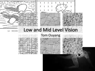
Low and Mid Level Vision Tom Ouyang. papers. “ Despite considerable progress in recent years, our understanding of the principles underlying visual perception remains primitive . Attempts to construct computer models for the interpretation of arbitrary scenes have

E N D
“Despite considerable progress in recent years, our understanding of the principles underlying visual perception remains primitive. Attempts to construct computer models for the interpretation of arbitrary scenes have resulted in such poor performance, limited range of abilities, and inflexibility that, were it not for the human existence proof, we might have been tempted long ago to conclude that high-performance, general-purpose vision is impossible.”
current machine vision • Works well in limited domains • Attempts to solve problems directly from intensity image • Jumps from pictorial features to descriptions of complete objects
human vision • General solution, works over large variations in viewing conditions • Reflectance and color are estimated over a wide range of illuminations • Shadows are usually easily distinguished from changes in reflectance • Surface shape is easily discerned regardless of illumination or surface markings
intrinsic images • Humans are very good at inferring intrinsic characteristics from intensity • Range • Orientation • Reflectance • Incident illumination • Even for new scenes unlike any seen before • Micrographs, abstract art, etc
value of intrinsic characteristics • 3-D structure of the scene • Navigation and manipulation • More invariant and distinguishing description • Simply perception • Scene partitioning • Viewpoint independent description of objects
value of intrinsic characteristics • 3-D structure of the scene • Navigation and manipulation • More invariant and distinguishing description • Simply perception • Scene partitioning • Viewpoint independent description of objects Alleviates many of the difficulties in current vision systems
approach a visual system, whether for an animal or a machine, should be organized around an initial level of domain-independent processing, the purpose of which is the recovery of intrinsic scene characteristics from image intensities
recovering intrinsic images • Is information in input intensity image sufficient? • Image formation: Intensity determined by three factors • Incident illumination • Local surface reflectance • Local surface orientation • Problem is ambiguous: must extract many attributes from single intensity value
lighting intensity example (simple case of ideally diffusing surface)
a solution for a simple world • Only hope of decoding the information is by making assumptions • Construct an idealized domain that… • is simple enough to exhaustively enumerate constraints and appearances • but complex enough for the recovery process to be non-trivial • Answer: world of colored Play-Doh
constraints • Surfaces are continuous • continuous distance and orientation • Surfaces are lambertian • perfectly diffusive reflection • no surface markings or textures • Uniform diffuse background lighting • Illumination from distant point source
illumination model “Sun and sky” • In shadowed areas • In illuminated areas
interesting properties • Image intensity is independent of viewing direction • surface is lambertian, so reflected light is distributed uniformly over a hemisphere • Image intensity is independent of viewing distance • surface area increases as density decreases
regions • For illuminated regions, variations in intensity due solely to variations in surface orientation • Since I0, I1, and R are constant • For shadowed regions, intensity is constant • Thus, we can catalog regions as either smoothly varying or constant
shadowed edges • difference only in illumination • constant intensity on shadowed side • varying intensity on illuminated side • shadow darker than illuminated region
surface (extremal) edges • local extremum of surface • where surface turns away from viewer • orientation normal to line of sight • adjacent regions independently illuminated
tangency test • For a surface boundary, orientation is constant. • Possible to determine reflectance at any point • Uniform reflectance assumption -> reflectance estimates much agree
junctions Two classes of (T) junctions • Occlusion • crossbar = extremal edge • stem = occluded edge • Cast Shadow • crossbar = extremal edge • stem = shadowed edge occlusion cast shadow
recovery using catalog • Detect edges in input intensity image • Determine intrinsic nature of regions and edges • Assign initial values for intrinsic characteristics • Propagate “boundary” values into interiors of regions (continuity assumption)
initializing intrinsic values • Interpret edges using constancy and tangency tests (shadow or surface) • Applied to adjacent regions • Initialize intrinsic values using edge table • Assign defaults for unspecified values
consistency • Establish consistency in intrinsic values • Constant reflectance (except at edges) • Continuous orientation (except at edges) • Continuous illumination (except in shadows) • Continuous distance (except at edges) • Implemented via asynchronous parallel processes • Continuity: Laplace’s equations for relaxation
computational model • Edges (Sweeping arrows) • Catalog and propagate to intrinsic images • Local (circles) • Modify intrinsic values • Intra-image continuity and limit constraints • Xs • insert and delete edge elements
impact and recent interest • Most papers seek to solve vision problems directly from the intensity image • Revival: recent methods in de-lighting produces reflectance and illumination image • Work remains on relaxation/propagation
“right” partition? • No single answer • Bayesian approach: Depends on prior world knowledge • Low Level: • coherence of brightness • color • texture • motion • Mid or High level • symmetries of objects
no right answer • Returning a tree instead of a flat partition • Come up with hierarchical partitions • From big picture downward
questions • Prior literature • Agglomerative/divisive clustering • Region based • MRF • What is the criterion for a good partition? • How can such a criterion be computed effectively?
graph theoretic approach • Graph theoretic formulation of grouping • points represented as undirected graph • edges connect every pair of nodes • weight on each edge is a function of the similarity between the two points • Grouping • Maximize similarity within sets • Minimize similarity across sets
graph cut • Definition: • Cut = total weight of edges removed • Optimal bi-partition is one that minimizes the cut value
minimum cut • Well studied problem: efficient algorithms exist for finding the minimum cut of a graph • (Wu and Leahy): proposed a clustering method based on this criterion • can be used to produce good segmentation on some images
minimum cut • Problem: • favors cutting smalls sets of isolated nodes • cut(A,B) increases with the number of edges going across the two partitions
n (normalized) -cut • Instead of looking at total edge weights… • compute cut cost as a fraction of total edge connections (total connection from A to all nodes in the graph)
n-cut • Partitions of small isolated points no longer have small Ncut value • cut is now a large percentage of total connections • Example: Min-cut 1 100% of total connections
n-assoc • We can define measure of normalized association within a group • Reflects how tightly node within groups are connected to each other
n-cut and n-assoc • Property: maximizing association and minimizing disassociation are identical
computing the optimal partition • Matrix formulation • We can rewrite Ncut(A,B) as:
matrix formulation (1+x)indicator for x>1 Nx1 vector of 1’s
matrix formulation • After a bit of vector algebra we have… • Rayleigh quotient
computing the optimal partition • Unfortunately problem is NP-complete • If we allow y to be real valued, we can approximate the solution by solving the equation: • Real-valued solution is the 2nd smallest eigenvector
computing the optimal partition • Higher eigenvectors optimally subpartition the first two parts • However, accumulated quantization errors makes them less reliable • Solution: restart the partitioning on each subgraph recursively
complexity • Finding eigenvectors for an n x n matrix: O(n3) • impractical for large images • Optimizations: • Make affinity matrix sparse, only local points are connected • Randomly selecting connections from neighborhood