Stepwise Multiple Regression

1. Stepwise Multiple Regression

2. Different Methods for Entering Variables in Multiple Regression • Different types of multiple regression are distinguished by the method for entering the independent variables into the analysis. • In standard (or simultaneous) multiple regression, all of the independent variables are entered into the analysis at the same. • In hierarchical (or sequential) multiple regression, the independent variables are entered in an order prescribed by the analyst. • In stepwise (or statistical) multiple regression, the independent variables are entered according to their statistical contribution in explaining the variance in the dependent variable. • No matter what method of entry is chosen, a multiple regression that includes the same independent variables and the same dependent variables will produce the same multiple regression equation. • The number of cases required for stepwise regression is greater than the number for the other forms. We will use the norm of 40 cases for each independent variable.

3. Purpose of Stepwise Multiple Regression • Stepwise regression is designed to find the most parsimonious set of predictors that are most effective in predicting the dependent variable. • Variables are added to the regression equation one at a time, using the statistical criterion of maximizing the R² of the included variables. • After each variable is entered, each of the included variables are tested to see if the model would be better off it were excluded. This does not happen often. • The process of adding more variables stops when all of the available variables have been included or when it is not possible to make a statistically significant improvement in R² using any of the variables not yet included. • Since variables will not be added to the regression equation unless they make a statistically significant addition to the analysis, all of the independent variable selected for inclusion will have a statistically significant relationship to the dependent variable. • An example of how SPSS does stepwise regression is shown below.

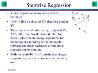
4. Stepwise Multiple Regression in SPSS • Each time SPSS includes or removes a variable from the analysis, SPSS considers it a new step or model, i.e. there will be one model and result for each variable included in the analysis. • SPSS provides a table of variables included in the analysis and a table of variables excluded from the analysis.  It is possible that none of the variables will be included.  It is possible that all of the variables will be included. • The order of entry of the variables can be used as a measure of relative importance. • Once a variable is included, its interpretation in stepwise regression is the same as it would be using other methods for including regression variables.

5. Pros and Cons of Stepwise Regression • Stepwise multiple regression can be used when the goal is to produce a predictive model that is parsimonious and accurate because it excludes variables that do not contribute to explaining differences in the dependent variable. • Stepwise multiple regression is less useful for testing hypotheses about statistical relationships. It is widely regarded as atheoretical and its usage is not recommended. • Stepwise multiple regression can be useful in finding relationships that have not been tested before. Its findings invite one to speculate on why an unusual relationship makes sense. • It is not legitimate to do a stepwise multiple regression and present the results as though one were testing a hypothesis that included the variables found to be significant in the stepwise regression. • Using statistical criteria to determine relationships is vulnerable to over-fitting the data set used to develop the model at the expense of generalizability. • When stepwise regression is used, some form of validation analysis is a necessity. We will use 75/25% cross-validation.

6. 75/25% Cross-validation • To do cross validation, we randomly split the data set into a 75% training sample and a 25% validation sample. We will use the training sample to develop the model, and we test its effectiveness on the validation sample to test the applicability of the model to cases not used to develop it. • In order to be successful, the follow two questions must be answers affirmatively: • Did the stepwise regression of the training sample produce the same subset of predictors produced by the regression model of the full data set? • If yes, compare the R2 for the 25% validation sample to the R2 for the 75% training sample. If the shrinkage (R2 for the 75% training sample - R2 for the 25% validation sample) is 2% (0.02) or less, we conclude that validation was successful. • Note: shrinkage may be a negative value, indicating that the accuracy rate for the validation sample is larger than the accuracy rate for the training sample. Negative shrinkage (increase in accuracy) is evidence of a successful validation analysis. • If the validation is successful, we base our interpretation on the model that included all cases.

7. IV1 IV2 DV DV Correlations between dependent variable and independent variables We have two independent variables, IV1 and IV2, which each have a relationship to the dependent variable. The areas of IV1 and IV2 which overlap with DV are r² values, i.e. the proportion of the dv that is explained by the iv. DV and IV1 are correlated at r = .70. The area of overlap is r² = .49. DV and IV2 are correlated at r = .40. The area of overlap is r² = .16.

8. IV1 IV2 Correlations between independent variables The two independent variables, IV1 and IV2, are correlated at r = .20. This correlation represents redundant information in the independent variables.

9. IV1 IV2 DV Variance in the dependent variable explained by the independent variables The variance explained in DV is divided into three areas. The total variance explained is the sum of the three areas. The green area is the variance in DV uniquely explained by IV1. The orange area is the variance in DV uniquely explained by IV2. The brown area is the variance in DV that is explained by both IV1 and IV2.

10. IV1 DV Correlations at step 1 of the stepwise regression Since IV1 had the stronger relationship with DV (.70 versus .40), it will be the variable entered first in the stepwise regression. As the only variable in the regression equation, it is given full credit (.70) for its relationship to DV. The partial correlation and the part correlation have the same value as the zero-order correlation at .70.

11. Change in variance explained when a second variable in included At step 2, IV2 enters the model, increasing the total variance explained from .49 to .56, an increase 0f .07. By itself, IV2 explained .16 of the variance in DV, but since it was itself correlated with IV1, a portion of what it could explain had already been attributed to IV1.

12. Differences in correlations when a second variable is entered While the zero-order correlations do not change, both the partial and the part correlations decrease. Partial correlation represents the relationship between the dependent variable and an independent variable when the relationship between the dependent variable and other independent variables has been removed from the variance of both the dependent and the independent variable. Part (or semi-partial) correlation is the portion of the total variance in the dependent variable that is by only that independent variable. The square of part correlation is the amount of change in R² by including this variable.

13. IV1 IV1 IV2 DV DV Zero-order, partial, and part correlations The zero-order correlation is based on the relationship between the independent variable and the dependent variable, ignoring all other independent variables. Part correlation for IV1 is the green area divided by all parts of DV, i.e. including areas associated with IV2. The partial correlation for IV1 is the green area divided by the area in DV and IV1 that is not part of IV2, i.e. green divided by green + yellow. NOTE: diagrams are scaled to r2 rather than r.

14. IV1 IV2 IV2 DV DV Zero-order, partial, and part correlations The partial correlation for IV2 is the green area divided by the area in DV and IV2 that is not part of IV2, i.e. orange divided by orange + yellow. The zero-order correlation is based on the relationship between the independent variable and the dependent variable, ignoring all other independent variables. Part correlation for IV2 is the orange area divided by all parts of DV, i.e. including areas associated with IV1.

15. How SPSS Stepwise Regression Chooses Variables - 1 We can use the table of correlations to identify which variable will be entered at the first step of the stepwise regression. The table of Correlations shows the the variable with the strongest individual relationship with the dependent variable is RACE OF HOUSEHOLD=WHITE, with a correlation of -.247. Provided that the relationship between this variable and the dependent variable is statistically significant, this will be the variable that enters first.

16. How SPSS Stepwise Regression Chooses Variables - 2 The correlation between RACE OF HOUSEHOLD=WHITE and importance of ethnic group to R is statistically significant at p < .001. It will be the first variable entered into the regression equation.

17. How SPSS Stepwise Regression Chooses Variables - 3 Model 1 contains the variable RACE OF HOUSEHOLD=WHITE, with a Multiple R of .247, producing an R² of .061 (.247²), which is statistically significant at p < .001. We cannot use the table of correlations to show which variable will be entered second, since the variable entered second must take into account its correlation to the independent variable entered first.

18. How SPSS Stepwise Regression Chooses Variables - 4 The table of Excluded Variables, however, shows the Partial Correlation between each candidate for entry and the dependent variable. In this example, RACE OF HOUSEHOLD=BLACK has the largest Partial Correlation (.252) and is statistically significant at p < .001, so it will be entered on the next step Partial correlation is a measure of the relationship of the dependent variable to an independent variable, where the variance explained by previously entered independent variables has been removed from both.

19. How SPSS Stepwise Regression Chooses Variables - 5 As expected, Model 2 contains the variable RACE OF HOUSEHOLD=WHITE and RACE OF HOUSEHOLD=BLACK. The R² for Model 2 increased by 0.059 to a total of .120. The increase in R² was statistically significant at p < .001.

20. How SPSS Stepwise Regression Chooses Variables - 6 The increase in R² of .059 is the square of the Part Correlation for RACE OF HOUSEHOLD=BLACK (.244² = 0.059). Part correlation, also referred to as semi-partial correlation, is the unique relationship between this independent variable and the dependent variable.

21. How SPSS Stepwise Regression Chooses Variables - 7 Partial Correlation Column Sig. Column In the table of Excluded Variables for model 2, the next largest partial correlation is HOW OFTEN R ATTENDS RELIGIOUS SERVICES at .149. This is the variable that will be added in Model 3 because the relationships is statistically significant at p = 0.32.

22. How SPSS Stepwise Regression Chooses Variables - 8 As expected, Model 3 contains the variable RACE OF HOUSEHOLD=WHITE and RACE OF HOUSEHOLD=BLACK, and HOW OFTEN R ATTENDS RELIGIOUS SERVICES . The R² for Model 3 increased by 0.019 to a total of .140. The increase in R² was statistically significant at p = .032.

23. How SPSS Stepwise Regression Chooses Variables - 9 Partial Correlation Column In the table of Excluded Variables for model 3, the next largest partial correlation is THINK OF SELF AS LIBERAL OR CONSERVATIVE at .089. Sig. Column However, the partial correlation is not significant (p=.203), so no additional variables will be added to the model.

24. What SPSS Displays when Nothing is Significant If none of the independent variables has a statistically significant relationship to the dependent variable, SPSS displays an empty table for Variables Entered/Removed.

25. The Problem in BlackBoard - 1 • The introductory problem statement tells us: • the data set to use: GSS2002_PrejudiceAndAltruism.SAV • the method for including variables in the regression • The dependent variable for the analysis • the list of independent variables that stepwise regression will select from

26. This Week’s Problems • The problems this week take the 13 questions on prejudice from the general social survey and explore the relationship of each to the demographic characteristics of age, education, income, political views (conservative versus liberal), religiosity (attendance at church), socioeconomic index, gender, and race. • I had no specific hypothesis about which demographic factors would be related to which question on prejudice, beyond an expectation that race would be a significant contributor to explaining differences on each of the questions. • My analyses were exploratory (to identify what demographic characteristics were associated with different aspects of prejudice) and, thus, appropriate for stepwise regression.

27. The Problem in BlackBoard - 2 In these problems, we will assume that our data satisfies the assumptions required by multiple regression without explicitly testing for it. We should recognize that failing to use a needed transformation could preclude a variable from being selected as a predictor. In your analyses, you would, of course, want to test for conformity to all of the assumptions.

28. The Problem in BlackBoard - 3 The next sequence of specific instructions tell us whether each variable should be treated as metric or non-metric, along with the reference category to use when dummy-coding non-metric variables. Though we will not use the script to test for assumptions, we can use it to do the dummy coding that we need for the problem.

29. The Problem in BlackBoard - 4 The next pair of instructions tell us the probability values to use for alpha for both the tests of statistical relationships and for the diagnostic tests.

30. The Problem in BlackBoard - 4 The final instruction tells us the random number seed to use in the validation analysis. If you do not use this number for the seed, it is likely that you will get different results from those shown in the feedback.

31. The Statement about Level of Measurement The first statement in the problem asks about level of measurement. Stepwise multiple regression requires the dependent variable and the metric independent variables be interval level, and the non-metric independent variables be dummy-coded if they are not dichotomous. The only way we would violate the level of measurement would be to use a nominal variable as the dependent variable, or to attempt to dummy-code an interval level variable that was not grouped.

32. Marking the Statement about Level of Measurement - 1 Stepwise multiple regression requires the dependent variable and the metric independent variables be interval level, and the non-metric independent variables be dummy-coded if they are not dichotomous. • Mark the check box as a correct statement because: • "Importance of ethnic identity" [ethimp] is ordinal level, but the problem calls for treating it as metric, applying the common convention of treating ordinal variables as interval level. • The metric independent variable "age" [age] was interval level, satisfying the requirement for independent variables. • The metric independent variable "highest year of school completed" [educ] was interval level, satisfying the requirement for independent variables. • "Income" [rincom98] is ordinal level, but the problem calls for treating it as metric, applying the common convention of treating ordinal variables as interval level.

33. Marking the Statement about Level of Measurement - 2 • In addition: • "Description of political views" [polviews] is ordinal level, but the problem calls for treating it as metric, applying the common convention of treating ordinal variables as interval level. • "Frequency of attendance at religious services" [attend] is ordinal level, but the problem calls for treating it as metric, applying the common convention of treating ordinal variables as interval level. • The metric independent variable "socioeconomic index" [sei] was interval level, satisfying the requirement for independent variables. • The non-metric independent variable "sex" [sex] was dichotomous level, satisfying the requirement for independent variables. • The non-metric independent variable "race of the household" [hhrace] was nominal level, but will satisfy the requirement for independent variables when dummy coded.

34. The Statement for Sample Size The statement for sample size indicates that the available data satisfies the requirement. Because of the tendency for stepwise regression to over-fit the data, we have a larger sample size requirement, i.e. 40 cases per independent variable (Tabachnick and Fidell, p. 117) To obtain the number of cases available for this analysis, we run the stepwise regression.

35. Using the Script to Create Dummy-coded Variables - 1 Before we can run the stepwise regression, we need to dummy code sex and race. We will use the script to create the dummy-coded variables. Select the Run Script command from the Utilities menu.

36. Using the Script to Create Dummy-coded Variables - 2 Navigate to the My Documents folder, if necessary. Highlight the script file SatisfyingRegressionAssumptionsWith MetricAndNonMetricVariables.SBS. Click on the Run button to open the script.

37. Using the Script to Create Dummy-coded Variables - 3 Move the non-metric variable "sex" [sex] to the list box for Non-metric independent variables list box. With the variable highlighted, select the reference category, 2=FEMALE from the Reference category drop down menu.

38. Using the Script to Create Dummy-coded Variables - 4 Move the non-metric variable "race of the household" [hhrace] to the list box for Non-metric independent variables list box. With the variable highlighted, select the reference category, 3=OTHER from the Reference category drop down menu. The OK button to run the regression is deactivated until we select a dependent variable.

39. Using the Script to Create Dummy-coded Variables - 5 We select the dependent variable "importance of ethnic identity" [ethimp], though since we are not going to interpret the output, we could select any variable. To have the script save the dummy-coded variables, clear the check box Delete variables created in this analysis.

40. Using the Script to Create Dummy-coded Variables - 6 Click on the OK button to run the regression, creating the dummy-coded variables as a by-product.

41. The Dummy-Coded Variables in the Data Editor If we scroll the variable list to the right, we see that the three dummy-coded variables have been added to the data set.

42. Run the Stepwise Regression - 1 To run the regression, select Regression > Linear from the Analyze menu.

43. Run the Stepwise Regression - 2 • Move the dependent variable • "importance of ethnic identity" [ethimp] • to the Dependent text box. • Move the independent variables: • "age" [age] • "highest year of school completed" [educ], • "income" [rincom98], • "description of political views" [polviews], • "frequency of attendance at religious services" [attend], • "socioeconomic index" [sei], • “survey respondents were male" [sex_1], • "survey respondents who were white" [hhrace_1], • "survey respondents who were black" [hhrace_2] • to the Independent(s) list box.

44. Run the Stepwise Regression - 3 The critical step to produce a stepwise regression is the selection of the method for entering variables. Select Stepwise from the Method drop down menu.

45. Run the Stepwise Regression - 4 Click on the Statistics button to specify additional output.

46. Run the Stepwise Regression - 5 • We mark the check boxes for optional statistics: • R squared change, • Descriptives, • Part and partial correlations, • Collinearity diagnostics, and • Durbin-Watson. Click on the Continue button to close the dialog box.

47. Run the Stepwise Regression - 6 Click on the OK button to produce the output.

48. Answering the Sample Size Question The analysis included 9 independent variables (6 metric independent variables plus 3 dummy-coded variables). The number of cases available for the analysis was 209, not satisfying the requirement for 360 cases based on the rule of thumb that the required number of cases for stepwise multiple regression should be 40 x the number of independent variables recommended by Tabachnick and Fidell (p. 117). We should consider mentioning the sample size issue as a limitation of the analysis.

49. Marking the Statement for Sample Size The check box is not marked because we did not satisfy the sample size requirement.

50. Statements about Variables Included in Stepwise Regression Three statements in the problem list different combinations of the variables included in the stepwise regression. To determine which is correct, we look at the table of Variables Entered and Removed in the SPSS output.