Stepwise Regression
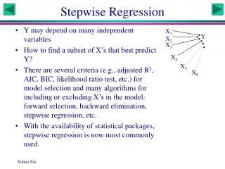
Stepwise Regression. Y may depend on many independent variables How to find a subset of X’s that best predict Y?

Stepwise Regression
E N D
Presentation Transcript
Stepwise Regression • Y may depend on many independent variables • How to find a subset of X’s that best predict Y? • There are several criteria (e.g., adjusted R2, AIC, BIC, likelihood ratio test, etc.) for model selection and many algorithms for including or excluding X’s in the model: forward selection, backward elimination, stepwise regression, etc. • With the availability of statistical packages, stepwise regression is now most commonly used. X1 Y X2 X3 X4 X5 X6
A Data Set for Multiple Regression Measurements on men involved in a physical fitness course at N. C. State University. Fitness is typically measured by oxygen intake rate (oxy) which is difficult (at least cumbersome) to measure. The study goal is to develop an equation to predict oxy based on exercise tests rather than on oxygen consumption measurements. The dataset has 31 observations. The variables in the data set are: age (in years) weight (in kg) oxy (oxygen intake rate, ml per kg body weight per minute) runtime (time to run 1.5 miles, in minutes) rstpulse (heart rate while resting) runpulse (heart rate while running, at the same time when oxygen rate was measured) maxpulse (maximum heart rate recorded while running). age weight oxy runtime rstpulse runpulse maxpulse; 44 89.47 44.609 11.37 62 178 182 40 75.07 45.313 10.07 62 185 185 44 85.84 54.297 8.65 45 156 168 . . . . . . .
Correlation matrix age weight oxy runtime rstpulse runpulse maxpulse age 1.00000 -0.23354 -0.30459 0.18875 -0.16410 -0.33787 -0.43292 0.2061 0.0957 0.3092 0.3777 0.0630 0.0150 weight -0.23354 1.00000 -0.16275 0.14351 0.04397 0.18152 0.24938 0.2061 0.3817 0.4412 0.8143 0.3284 0.1761 oxy -0.30459 -0.16275 1.00000 -0.86219 -0.39936 -0.39797 -0.23674 0.0957 0.3817 <.0001 0.0260 0.0266 0.1997 runtime 0.18875 0.14351 -0.86219 1.00000 0.45038 0.31365 0.22610 0.3092 0.4412 <.0001 0.0110 0.0858 0.2213 rstpulse -0.16410 0.04397 -0.39936 0.45038 1.00000 0.35246 0.30512 0.3777 0.8143 0.0260 0.0110 0.0518 0.0951 runpulse -0.33787 0.18152 -0.39797 0.31365 0.35246 1.00000 0.92975 0.0630 0.3284 0.0266 0.0858 0.0518 <.0001 maxpulse -0.43292 0.24938 -0.23674 0.22610 0.30512 0.92975 1.00000 0.0150 0.1761 0.1997 0.2213 0.0951 <.0001
Scatterplot matrix proccorr; var age weight oxy runtime rstpulse runpulse maxpulse ; run; procsgscatter; title "Scatterplot Matrix"; /*Create the scatter plot matrix. */ matrix age weight oxy runtime rstpulse runpulse maxpulse ; run; What is the advantage of a scatterplot matrix over a correlation matrix?
SAS program: stepwise regression data fitness; input age weight oxy runtime rstpulse runpulse maxpulse @@; cards; 44 89.47 44.609 11.37 62 178 182 40 75.07 45.313 10.07 62 185 185 44 85.84 54.297 8.65 45 156 168 42 68.15 59.571 8.17 40 166 172 38 89.02 49.874 9.22 55 178 180 47 77.45 44.811 11.63 58 176 176 40 75.98 45.681 11.95 70 176 180 43 81.19 49.091 10.85 64 162 170 44 81.42 39.442 13.08 63 174 176 38 81.87 60.055 8.63 48 170 186 44 73.03 50.541 10.13 45 168 168 45 87.66 37.388 14.03 56 186 192 45 66.45 44.754 11.12 51 176 176 47 79.15 47.273 10.60 47 162 164 54 83.12 51.855 10.33 50 166 170 49 81.42 49.156 8.95 44 180 185 51 69.63 40.836 10.95 57 168 172 51 77.91 46.672 10.00 48 162 168 48 91.63 46.774 10.25 48 162 164 49 73.37 50.388 10.08 67 168 168 57 73.37 39.407 12.63 58 174 176 54 79.38 46.080 11.17 62 156 165 52 76.32 45.441 9.63 48 164 166 50 70.87 54.625 8.92 48 146 155 51 67.25 45.118 11.08 48 172 172 54 91.63 39.203 12.88 44 168 172 51 73.71 45.790 10.47 59 186 188 57 59.08 50.545 9.93 49 148 155 49 76.32 48.673 9.40 56 186 188 48 61.24 47.920 11.50 52 170 176 52 82.78 47.467 10.50 53 170 172 ; procreg; model oxy=age weight runtime runpulse rstpulse maxpulse / selection=stepwise; run; procglmselect; model oxy=age weight runtime runpulse rstpulse maxpulse / selection=stepwise; run; procglmselect; model oxy=age weight runtime runpulse rstpulse maxpulse / selection=stepwise (select=SL SLE=0.2 SLS=0.15); run; Default criterion: p = 0.15 Default cteririon is Schwarz Bayesian information criterion (SBC) Significance Level entry SL stay SL
Stepwise Reg: Steps 1 Variable runtime Entered: R-Square = 0.7434 and C(p) = 13.6988 Analysis of Variance Sum of Mean Source DF Squares Square F Value Pr > F Model 1 632.90010 632.90010 84.01 <.0001 Error 29 218.48144 7.53384 Corrected Total 30 851.38154 Parameter Standard Variable Estimate Error Type II SS F Value Pr > F Intercept 82.42177 3.85530 3443.36654 457.05 <.0001 runtime -3.31056 0.36119 632.90010 84.01 <.0001 The statistic Cp was introduced by C. L. Mallows who credited the conception of the statistic to discussions with Cuthbert Daniel (hence the C to honor the latter). The best model has the smallest Cp value.
Stepwise Reg: Step 2-3 Variable age Entered: R-Square = 0.7642 and C(p) = 12.3894 Analysis of Variance Sum of Mean Source DF Squares Square F Value Pr > F Model 2 650.66573 325.33287 45.38 <.0001 Error 28 200.71581 7.16842 Corrected Total 30 851.38154 Parameter Standard Variable Estimate Error Type II SS F Value Pr > F Intercept 88.46229 5.37264 1943.41071 271.11 <.0001 age -0.15037 0.09551 17.76563 2.48 0.1267 runtime -3.20395 0.35877 571.67751 79.75 <.0001 Variable runpulse Entered: R-Square = 0.8111 and C(p) = 6.9596 Analysis of Variance Sum of Mean Source DF Squares Square F Value Pr > F Model 3 690.55086 230.18362 38.64 <.0001 Error 27 160.83069 5.95669 Corrected Total 30 851.38154 Parameter Standard Variable Estimate Error Type II SS F Value Pr > F Intercept 111.71806 10.23509 709.69014 119.14 <.0001 age -0.25640 0.09623 42.28867 7.10 0.0129 runtime -2.82538 0.35828 370.43529 62.19 <.0001 runpulse -0.13091 0.05059 39.88512 6.70 0.0154
Stepwise Reg: Step 4 Variable maxpulse Entered: R-Square = 0.8368 and C(p) = 4.8800 Analysis of Variance Sum of Mean Source DF Squares Square F Value Pr > F Model 4 712.45153 178.11288 33.33 <.0001 Error 26 138.93002 5.34346 Corrected Total 30 851.38154 Parameter Standard Variable Estimate Error Type II SS F Value Pr > F Intercept 98.14789 11.78569 370.57373 69.35 <.0001 age -0.19773 0.09564 22.84231 4.27 0.0488 runtime -2.76758 0.34054 352.93570 66.05 <.0001 runpulse -0.34811 0.11750 46.90089 8.78 0.0064 maxpulse 0.27051 0.13362 21.90067 4.10 0.0533 All vari ables left in the model are significant at the 0.1500 level. No other variable met the 0.1500 significance level for entry into the model.
Run SAS and explain output procglmselect; model oxy=age weight runtime runpulse rstpulse maxpulse / selection=stepwise; run; procglmselect; model oxy=age weight runtime runpulse rstpulse maxpulse / selection=stepwise (select=SL SLE=0.2 SLS=0.15); run;
Criteria used in model selection • Ra2 • Cp • SBC (BIC) • AIC • Significance level Xia, X. 2009. Information-theoretic indices and an approximate significance test for testing the molecular clock hypothesis with genetic distances. Molecular Phylogenetics and Evolution 52:665-676. Burnham, K. P. and D. R. Anderson. 2002 Model selection and multimodel inference: a practical information-theoretic approach. 2nd ed. Springer. (Best book on model selection)
Revisiting Liquor and Church Data Data Mydata; input Liquor Church CitySize; cards; 10041.7887 1 10000 20096.1752 3 20000 10041.7887 2 10000 . . ; proc reg; model Liquor=Church CitySize / SS1; run; proc reg; model Liquor=CitySize Church/ SS1; run; Liquor Cons N. Church City Size 10041.7887 1 10000 20096.1752 3 20000 10041.7887 2 10000 30083.8478 3 30000 20096.1752 1 20000 40014.8096 5 40000 50060.0323 4 50000 60043.2171 6 60000 20096.1752 3 20000 50060.0323 4 50000 10041.7887 2 10000 10041.7887 1 10000 70096.1250 8 70000 50060.0323 2 50000 80064.3763 9 80000 90094.3248 9 90000 100034.3940 10 100000 110066.0155 10 110000
SAS Output Sum of Mean Source DF Squares Square F Value Prob>F Model 2 18429734317 9214867158.5 12417776.418 0.0001 Error 15 11131.05944 742.07063 C Total 17 18429745448 When CHURCH is entered first: Variable DF Type I SS INTERCEP 1 38376770918 CHURCH 1 16456929141 CITYSIZE 1 1972805176 When CITYSIZE is entered first: Variable DF Type I SS INTERCEP 1 38376770918 CITYSIZE 1 18429734316 CHURCH 1 0.929861 • From a statistical point of view, the regression model including CITYSIZE and excluding CHURCH is better than that including CHURCH and excluding CITISIZE. • What should we do if CHURCH is in fact a better predictor of Liquor consumption than CITISIZE?
The two purposes of regression • Predictive: find the best set of X’s to predict Y • Functional characterization of the true (causal) relationship between Y and X’s.