linear algebraic systems i
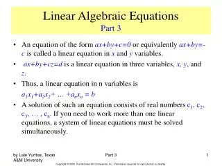
Fundamental Theorem. Linear algebraic systemConsistencyThe system has solutions if and only if the matrices A and have the same rank rUniquenessThe system has a single solution if and only if both matrices have rank r = nInfinitely many solutionsThe system has infinitely many solutions if and only if both matrices have rank r < n.

linear algebraic systems i
E N D
Presentation Transcript
1. Linear Algebraic Systems I Existence and uniqueness of solutions
Determinants and matrix inverses
Gauss-Jordan elimination
Ill-conditioned matrices
3. Implications Homogeneous system
Trivial solution: x = 0
Nontrivial solutions exist if and only if rank(A) < n
Nontrivial solutions are said to be contained in the null space of A
Nonhomogeneous system
If the system is consistent, then all solutions can be represented as x = x0+xh
x0 is a particular solution of the nonhomogeneous system
xh is any solution of the homogeneous system
4. Fundamental Theorem Examples Unique solution
Infinitely many solutions
No solutions
5. Determinants Only applicable to square matrices
Notation: det(A), |A|
2x2 matrix
3x3 matrix
More general formulas based on cofactors are presented in the text
6. Determinant Examples By hand
Using Matlab
>> A=[1 2; 3 4];
>> det(A)
ans = -2
>> A=[1 2 3;4 5 6;7 8 9];
>> det(A)
ans = 0
7. Properties of Determinants |A| = |AT|
Diagonal & triangular matrices
Products: |AB| = |A||B|
A zero column or row produces a zero determinant
Linearly dependent rows or columns produce a zero determinant
A square matrix A has full rank n if and only if |A| is non-zero
8. Matrix Inverse Definition
Assume A is a nxn matrix
The inverse of A is denoted A-1
The inverse satisfies the equations:
Existence & uniqueness
The inverse exists if and only if:
If A has an inverse, then the inverse is unique
Concepts
Singular matrix: A-1 does not exist, det(A) = 0, rank(A) < n
Nonsingular matrix: A-1 exists, det(A) non-zero, rank(A) = n
If rank(A) < n, the matrix is said to rank deficient
9. Special Cases 2x2 matrix
Diagonal matrix
Product of square matrices
10. Gauss-Jordan Elimination Method to compute A-1 using row operations
Form augmented matrix
Eliminate first entry in last two rows
11. Gauss-Jordan Elimination Eliminate x2 entry from third row
Make the diagonal elements unity
12. Gauss-Jordan Elimination cont. Eliminate first two entries in third column
Obtain identity matrix
Matrix inverse
13. Gauss-Jordan Elimination cont. Verify result
14. Using the Matrix Inverse Linear algebraic equation system: Ax = b
Assume A is a non-singular matrix
Solution
Example
15. Matlab Examples >> A=[-1 1 2; 3 -1 1; -1 3 4];
>> inv(A)
ans =
-0.7000 0.2000 0.3000
-1.3000 -0.2000 0.7000
0.8000 0.2000 -0.2000
>> A=[1 2; 3 5];
>> b=[1; 2];
>> x=inv(A)*b
x =
-1.0000
1.0000
16. Ill-Conditioned Matrices Matrix inversion: Ax = b ? x = A-1b
Assume A is a perfectly known matrix
Consider b to be obtained from measurement with some uncertainty
Terminology
Well-conditioned problem: �small� changes in the data b produce �small� changes in the solution x
Ill-conditioned problem: �small� changes in the data b produce �large� changes in the solution x
Ill-conditioned matrices
Caused by nearly linearly dependent equations
Characterized by nearly singular A matrix
Solution is not reliable
Common problem for large algebraic systems
Ill-conditioning quantified by the condition number (covered later)
17. Ill-Conditioned Matrix Example Example
e represents measurement error in b2
Two rows (columns) are nearly linearly dependent
Analytical solution
10% error (e = 0.1)
18. Matlab Example >> A=[1 2; 3 5];
>> cond(A)
ans = 38.9743 (well conditioned)
>> A=[0.9999 -1.0001; 1 -1];
>> cond(A)
ans = 2.0000e+004 (poorly conditioned)
>> b=[1; 1.1]
>> x=inv(A)*b
x =
500.5500
499.4500