Nonlinear Algebraic Systems
Nonlinear Algebraic Systems. Iterative solution methods Fixed-point iteration Newton-Raphson method Secant method Matlab tutorial Matlab exercise. Single Nonlinear Equation. Nonlinear algebraic equation: f ( x ) = 0 Analytical solution rarely possible Need numerical techniques

Nonlinear Algebraic Systems
E N D
Presentation Transcript
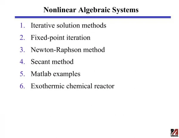
Nonlinear Algebraic Systems • Iterative solution methods • Fixed-point iteration • Newton-Raphson method • Secant method • Matlab tutorial • Matlab exercise
Single Nonlinear Equation • Nonlinear algebraic equation: f(x) = 0 • Analytical solution rarely possible • Need numerical techniques • Multiples solutions may exist • Iterative solution • Start with an initial guess x0 • Algorithm generates x1 from x0 • Repeat to generate sequence x0, x1, x2, … • Assume sequence convergences to solution • Terminate algorithm at iteration N when: • Many iterative algorithms available • Fixed-point iteration, Newton-Raphson method, secant method
Fixed-Point Iteration • Formulation of iterative equation • A solution of x = g(x) is called a fixed point • Convergence • The iterative process is convergent if the sequence x0, x1, x2, … converges: • Let x = g(x) have a solution x = s and assume that g(x) has a continuous first-order derivative on some interval J containing s, then the fixed-point iteration converges for any x0 in J & the limit of the sequence {xn} is s if: • A function satisfying the theorem is called a contraction mapping: • K determines the rate of convergence
Newton-Raphson Method • Iterative equation derived from first-order Taylor series expansion • Algorithm • Input data: f(x),df(x)/dx, x0, tolerance (d), maximum number of iterations (N) • Given xn, compute xn+1 as: • Continue until | xn+1-xn| < d|xn| or n = N
Convergence of the Newton-Raphson Method • Order • Provides a measure of convergence rate • Newton-Raphson method is second-order • Assume f(x) is three times differentiable, its first- and second-order derivatives are non-zero at the solution x= s & x0 is sufficiently close to s, then the Newton method is second-order & exhibit quadratic converge to s • Caveats • The method can converge slowly or even diverge for poorly chosen x0 • The solution obtained can depend on x0 • The method fails if the first-order derivative becomes zero (singularity)
Secant Method • Motivation • Evaluation of df/dx may be computationally expensive • Want efficient, derivative-free method • Derivative approximation • Secant algorithm • Convergence • Superlinear: • Similar to Newton-Raphson (m = 2)
Matlab Tutorial • Solution of nonlinear algebraic equations with Matlab • FZERO – scalar nonlinear zero finding • Matlab function for solving a single nonlinear algebraic equation • Finds the root of a continuous function of one variable • Syntax: x = fzero(‘fun’,xo) • ‘fun’ is the name of the user provided Matlab m-file function (fun.m) that evaluates & returns the LHS of f(x) = 0. • xo is an initial guess for the solution of f(x) = 0. • Algorithm uses a combination of bisection, secant, and inverse quadratic interpolation methods.
Matlab Tutorial cont. • Solution of a single nonlinear algebraic equation: • Write Matlab m-file function, fun.m: • Call fzero from the Matlab command line to find the solution: • Different initial guesses, xo, can give different solutions: >> xo = 0; >> fzero('fun',xo) ans = 0.5376 >> fzero('fun',4) ans = 3.4015 >> fzero('fun',1) ans = 1.2694
Nonisothermal Chemical Reactor • Reaction: A B • Assumptions • Pure A in feed • Perfect mixing • Negligible heat losses • Constant properties (r, Cp, DH, U) • Constant cooling jacket temperature (Tj) • Constitutive relations • Reaction rate/volume: r = kcA= k0exp(-E/RT)cA • Heat transfer rate: Q = UA(Tj-T)
Model Formulation • Mass balance • Component balance • Energy balance
Matlab Exercise • Steady-state model • Parameter values • k0 = 3.493x10⁷ h-1, E = 11843 kcal/kmol • (-DH) = 5960 kcal/kmol, rCp = 500 kcal/m3/K • UA = 150 kcal/h/K, R = 1.987 kcal/kmol/K • V = 1 m3, q =1 m3/h, • CAf = 10 kmol/m3, Tf= 298 K, Tj = 298 K. • Problem • Find the three steady-state points:
Matlab Tutorial cont. • FSOLVE – multivariable nonlinear zero finding • Matlab function for solving a system of nonlinear algebraic equations • Syntax: x = fsolve(‘fun’,xo) • Same syntax as fzero, but x is a vector of variables and the function, ‘fun’, returns a vector of equation values, f(x). • Part of the Matlab Optimization toolbox • Multiple algorithms available in options settings (e.g. trust-region dogleg, Gauss-Newton, Levenberg-Marquardt)
Matlab Exercise: Solution with fsolve • Syntax for fsolve • x = fsolve('cstr',xo,options) • 'cstr' – name of the Matlab m-file function (cstr.m) for the CSTR model • xo – initial guess for the steady state, xo = [CA T] '; • options – Matlab structure of optimization parameter values created with the optimset function • Solution for first steady state, Matlab command line input and output: >> xo = [10 300]'; >> x = fsolve('cstr',xo,optimset('Display','iter')) Norm of First-order Trust-region Iteration Func-count f(x) step optimality radius 0 3 1.29531e+007 1.76e+006 1 1 6 8.99169e+006 1 1.52e+006 1 2 9 1.91379e+006 2.5 7.71e+005 2.5 3 12 574729 6.25 6.2e+005 6.25 4 15 5605.19 2.90576 7.34e+004 6.25 5 18 0.602702 0.317716 776 7.26 6 21 7.59906e-009 0.00336439 0.0871 7.26 7 24 2.98612e-022 3.77868e-007 1.73e-008 7.26 Optimization terminated: first-order optimality is less than options.TolFun. x = 8.5637 311.1702
Matlab Exercise: cstr.m functionf = cstr(x) ko = 3.493e7; E = 11843; H = -5960; rhoCp = 500; UA = 150; R = 1.987; V = 1; q = 1; Caf = 10; Tf = 298; Tj = 298; Ca = x(1); T = x(2); f(1) = q*(Caf - Ca) - V*ko*exp(-E/R/T)*Ca; f(2) = rhoCp*q*(Tf - T) + -H*V*ko*exp(-E/R/T)*Ca + UA*(Tj-T); f=f';