Multiprocessors
Multiprocessors Processor Performance We have looked at various ways of increasing a single processor performance (Excluding VLSI techniques): Pipelining ILP Superscalers Out-of-order execution (Scoreboarding) VLIW Cache (L1, L2, L3) Interleaved memories


Multiprocessors
E N D
Presentation Transcript
Processor Performance • We have looked at various ways of increasing a single processor performance (Excluding VLSI techniques): • Pipelining • ILP • Superscalers • Out-of-order execution (Scoreboarding) • VLIW • Cache (L1, L2, L3) • Interleaved memories • Compilers (Loop unrolling, branch prediction, etc.) • RAID • Etc … • However, quite often even the best microprocessors are not good enough for certain applications !!!
Example: How far will ILP go? • Infinite resources and fetch bandwidth, perfect branch prediction and renaming
The need for High-Performance ComputersJust some examples • Automotive design: • Major automotive companies use large systems (500+ CPUs) for: • CAD-CAM, crash testing, structural integrity and aerodynamics. • Savings: approx. $1 billion per company per year. • Semiconductor industry: • Semiconductor firms use large systems (500+ CPUs) for • device electronics simulation and logic validation • Savings: approx. $1 billion per company per year. • Airlines: • System-wide logistics optimization systems on parallel systems. • Savings: approx. $100 million per airline per year.
structural biology vehicle dynamics pharmaceutical design 72-hour weather 48-hour weather chemical dynamics 3D plasma modelling 2D airfoil oil reservoir modelling Grand Challenges 1 TB 100 GB 10 GB 1 GB Storage Requirements 100 MB 10 MB 100 MFLOPS 1GFLOPS 10 GFLOPS 100 GFLOPS 1 TFLOPS Computational Performance Requirements
Global Climate Modelling • Example: Weather Forecasting with 3D Grid around the Earth: • Climate is a function of 4 arguments • Approach: • Discretize the domain, e.g., a measurement point every 1 km • Devise an algorithm to predict weather at time t+1 given t Climate(longitude, latitude, elevation, time) • Which returns a vector of 6 values Temperature, pressure, humidity, and wind velocity • 1 Kilometre Cells • 100 operations/cell • 1 minute time step
Multiprocessing • Multiprocessing (Parallel Processing): Concurrent execution of tasks (programs) using multiple computing, memory and interconnection resources. • Use multiple resources to solve problems faster. • Using multiple processors to solve a single problem • Divide problem into many small pieces • Distribute these small problems to be solved by multiple processors simultaneously
Multiprocessing • For the last 30+ years multiprocessing has been seen as the best way to produce orders of magnitude performance gains. • Double the number of processors, get double performance (less than 2 times the cost). • It turns out that the ability to develop and deliver software for multiprocessing systems has been the impediment to wide adoption.
Performance Potential Using Multiple Processors • Amdahl's Law is pessimistic (in this case) • Let s be the serial part • Let p be the part that can be parallelized n ways • Serial: SSPPPPPP • 6 processors: SSP • P • P • P • P • P • Speedup = 8/3 = 2.67 • T(n) = • As n , T(n) • Pessimistic 1 s+p/n 1 s
Performance Potential: An other view • Gustafson view (more widely adopted for multiprocessors) • Parallel portion increases as the problem size increases • Serial time fixed (at s) • Parallel time proportional to problem size (true most of the time) • Old Serial: SSPPPPPP • 6 processors: SSPPPPPP • PPPPPP • PPPPPP • PPPPPP • PPPPPP • PPPPPP • Hypothetical Serial: • SSPPPPPP PPPPPP PPPPPP PPPPPP PPPPPP PPPPPP • Speedup = (8+5*6)/8 = 4.75 • T'(n) = s + n*p; T'() !!!!
TOP 5 Most Powerful computers in the world – must be multiprocessors http://www.top500.org/
Multiprocessing (usage) • Multiprocessor systems are being used for a wide variety of uses. • Redundant processing (safeguard) – fault tolerance. • Multiprocessor systems – increase throughput • Many tasks (no communication between them) • Multi-user departmental, enterprise and web servers. • Parallel processor systems – decrease execution time. • Execute large-scale applications in parallel.
Multiprocessing • Multiple resources • Computers (e.g., clusters of PCs) • CPU (e.g., shared memory computers) • ALU (e.g., multiprocessors within a single chips) • Memory • Interconnect • Tasks • Programs • Procedures • Instructions Different combinations result in different systems. Coarse-grain Fine-grain
Why did the popularity of Multiprocessors slowed down compared to the 90s • The ability to develop and deliver software for multiprocessing systems has been the impediment to wide adoption – the goal was to make programming transparent to the user (e.g., pipelining) which never happened. However, there have a lot of advances here. • The tremendous advances of microprocessors (doubling in performance every 2 years) was able to satisfy the need of 99% of the applications • It did not make a business case: vendors were only able to sell few parallel computers (< 200). As a result, they were not able to invest in designing cheap and powerful multiprocessors • Most parallel computer vendors went bunkrupt by the mid-90s – there was no business.
Flynn’s Taxonomy of Computing • SISD (Single Instruction, Single Data): • Typical uniprocessor systems that we’ve studied throughout this course. • Uniprocessor systems can time share and still be SISD. • SIMD (Single Instruction, Multiple Data): • Multiple processors simultaneously executing the same instruction on different data. • Specialized applications (e.g., image processing). • MIMD (Multiple Instruction, Multiple Data): • Multiple processors autonomously executing different instructions on different data. • Keep in mind that the processors are working together to solve a single problem.
SIMD Parallel Computing It can be a stand-alone multiprocessor Or Embedded in a single processor for specific applications (MMX)
SIMD Applications • Applications: • Database, image processing, and signal processing. • Image processing maps very naturally onto SIMD systems. • Each processor (Execution unit) performs operations on a single pixel or neighborhood of pixels. • The operations performed are fairly straightforward and simple. • Data could be streamed into the system and operated on in real-time or close to real-time.
SIMD Operations • Image processing on SIMD systems. • Sequential pixel operations take a very long time to perform. • A 512x512 image would require 262,144 iterations through a sequential loop with each loop executing 10 instructions. That translates to 2,621,440 clock cycles (if each instruction is a single cycle) plus loop overhead. Each pixel is operated on sequentially one after another. 512x512 image
SIMD Operations • Image processing on SIMD systems. • On a SIMD system with 64x64 processors (e.g., very simple ALUs) the same operations would take 640 cycles, where each processor operates on an 8x8 set of pixels plus loop overhead. Each processor operates on an 8x8 set of pixels in parallel. Speedup due to parallelism: 2,621,440/640 = 4096 = 64x64 (number of proc.) loop overhead ignored. 512x512 image
SIMD Operations • Image processing on SIMD systems. • On a SIMD system with 512x512 processors (which is not unreasonable on SIMD machines) the same operation would take 10 cycles. Each processor operates on a single pixel in parallel. Speedup due to parallelism: 2,621,440/10 = 262,144 = 512x512 (number of proc.)! 512x512 image Notice no loop overhead!
Pentium MMX MultiMedia eXtentions • 57 new instructions • Eight 64-bit wide MMX registers • First available in 1997 • Supported on: • Intel Pentium-MMX, Pentium II, Pentium III, Pentium IV • AMD K6, K6-2, K6-3, K7 (and later) • Cyrix M2, MMX-enhanced MediaGX, Jalapeno (and later) • Gives a large speedup in many multimedia applications
MMX SIMD Operations • Example: consider an image pixel data represented as bytes. • with MMX, eight of these pixels can be packed together in a 64-bit quantity and moved into an MMX register • MMX instruction performs the arithmetic or logical operation on all eight elements in parallel • PADD(B/W/D): Addition PADDB MM1, MM2 adds 64-bit contents of MM2 to MM1, byte-by-byte any carries generated are dropped, e.g., byte A0h + 70h = 10h • PSUB(B/W/D): Subtraction
MMX: Image Dissolve Using Alpha Blending • Example: MMX instructions speed up image composition • A flower will dissolve a swan • Alpha (a standard scheme) determines the intensity of the flower • The full intensity, the flower’s 8-bit alpha value is FFh, or 255 • The equation below calculates each pixel: Result_pixel =Flower_pixel *(alpha/255) + Swan_pixel * [1-(alpha/255)] For alpha 230, the resulting pixel is 90% flower and 10% swan
SIMD Multiprocessing • It is easy to write applications for SIMD processors • The applications are limited (image processing, computer vision, etc.) • It is frequently used to speed specific applications (e.g., graphics co-processor in SGI computers) • In the late 80s and early 90s, many SIMD machines were commercially available (e.g., Connection machine has 64K ALUs, and MasPar has 16K ALUs)
Flynn’s Taxonomy of Computing • MIMD (Multiple Instruction, Multiple Data): • Multiple processors autonomously executing different instructions on different data. • Keep in mind that the processors are working together to solve a single problem. • This is a more general form of multiprocessing, and can be used in numerous applications
MIMD Architecture Instruction Stream A Instruction Stream C Instruction Stream B Unlike SIMD, MIMD computer works asynchronously. • Shared memory (tightly coupled) MIMD • Distributed memory (loosely coupled) MIMD Data Output stream A Data Input stream A Processor A Data Output stream B Processor B Data Input stream B Data Output stream C Processor C Data Input stream C
Shared Memory Multiprocessor Processor Processor Processor Processor Registers Registers Registers Registers Caches Caches Caches Caches Chipset Memory • Memory: centralized with Uniform Memory Access time(“uma”) and bus interconnect, I/O • Examples: Sun Enterprise 6000, SGI Challenge, Intel SystemPro Disk & other IO
Shared Memory Programming Model Processor Memory System Process Process load(X) store(X) X Shared variable
Shared Memory Model Virtual address spaces for a collection of processes communicating via shared addresses Machine physical address space Pn private Load Common physical addresses Store Shared portion of address space P2 private P1 private Private portion of address space P0 private
P P P P $ $ $ $ MEM Cache Coherence Problem • Processor 3 does not see the value written by processor 0 W: X = 17 R: X R: X X:17 X:42 X:42 X:42
P P P P $ $ $ $ MEM Write Through does not help • Processor 3 sees 42 in cache (does not get the correct value (17) from memory. W: X = 17 R: X R: X R: X X:17 X:17 X:42 X:42 X:42
P P 1 n Switch (Interleaved) First-level $ (Interleaved) Main memory Shared Cache One Solution: Shared Cache Advantages • Cache placement identical to single cache • only one copy of any cached block Disadvantages • Bandwidth limitation
Limits of Shared Cache Approach Assume: 1 GHz processor w/o cache => 4 GB/s inst BW per processor (32-bit) => 1.2 GB/s data BW at 30% load-store Need 5.2 GB/s of bus bandwidth per processor! • Typical bus bandwidth can hardly support one processor I/O MEM ° ° ° MEM 140 MB/s ° ° ° cache cache 5.2 GB/s PROC PROC
State Address Data Distributed Cache: Snoopy Cache-Coherence Protocols • Bus is a broadcast medium & caches know what they have • bus protocol: arbitration, command/addr, data => Every device observes every transaction
Snooping Cache Coherency • Cache Controller “snoops” all transactions on the shared bus • A transaction is a relevant transaction if it involves a cache block currently contained in this cache • take action to ensure coherence (invalidate, update, or supply value)
Hardware Cache Coherence • write-invalidate • write-update (also called distributed write) memory invalidate --> ICN X -> X’ X -> Inv X -> Inv . . . . . memory update --> ICN X -> X’ X -> X’ X -> X’ . . . . .
Limits of Bus-Based Shared Memory Assume: 1 GHz processor w/o cache => 4 GB/s inst BW per processor (32-bit) => 1.2 GB/s data BW at 30% load-store Suppose 98% inst hit rate and 95% data hit rate => 80 MB/s inst BW per processor => 60 MB/s data BW per processor • 140 MB/s combined BW Assuming 1 GB/s bus bandwidth \ 8 processors will saturate the memory bus I/O MEM ° ° ° MEM 140 MB/s ° ° ° cache cache 5.2 GB/s PROC PROC
Intel Pentium Pro Quad: Shared Bus Multiptocessor for the masses: • Uses Snoopy cache protocol
Scalable Shared Memory ArchitecturesCrossbar Switch Used in SUN entreprise 10000 Mem Mem Mem Mem Cache Cache I/O I/O P P
Scalable Shared Memory Architectures • Used in IBM SP Multiprocessor P M 000 0 0 P M 001 1 1 P M 010 2 2 1 P M 011 3 3 P M 100 4 4 1 P M 101 5 5 P M 110 6 6 0 P M 111 7 7
P P 1 n Switch (Interleaved) P First-level $ P n 1 $ $ (Interleaved) Main memory Inter connection network Mem Mem Approaches to Building Parallel Machines Scale Shared Cache P P n 1 $ $ Mem Mem Inter connection network Distributed Memory