Download
1 / 39
390 likes | 727 Vues
Ecology = Scientific study of natural communities. Experimental and observational tests. are tested by. Process. provisionally accept, revise or reject. Predictions. begets. lead to. Hypotheses. Pattern. delimit. suggest. made of. Observations. Principles.

E N D
Ecology = Scientific study of natural communities Experimental and observational tests are tested by Process provisionally accept, revise or reject Predictions begets lead to Hypotheses Pattern delimit suggest made of Observations Principles
Types of Terrestrial Ecosystems • Biomes are major groupings of plant and animal communities defined by a dominant vegetation type. • Each biome is associated with a distinctive set of abiotic conditions. • The type of biome present in a terrestrial region depends on climate—the prevailing, long-term weather conditions found in an area. • Weather consists of the specific short-term atmospheric conditions of temperature, moisture, sunlight, and wind.
Distinct Biomes Are Found throughout the World Barrow Dawson Chicago Konza Prairie Yuma Belém
Solar Radiation per Unit Area Declines with Increasing Latitude North pole Small amount of sunlight per unit area Low angle of incoming sunlight Moderate angle of incoming sunlight Sunlight directly overhead Large amount of sunlight per unit area
Global Air Circulation Patterns Affect Rainfall Circulation cells exist at the equator … Atmosphere (not to scale) Hadley cell Warm air rises and cools, dropping rain Hadley cell Cooled air is pushed poleward Dense, dry air descends, warms, and absorbs moisture
Global Air Circulation Patterns Affect Rainfall … and at higher latitudes. There are three circulation cells in the Northern Hemisphere There are also three circulation cells in the Southern Hemisphere (draw them in)
Figure 50-12 Tropical wet forests are extremely rich in species
Figure 50-14 Saguaro cacti are a prominent feature of the Sonoran Desert in the southwestern part of North America
Figure 50-16 Grasses are the dominant lifeform in prairies and steppes
Figure 50-18 Temperate forests are dominated by broad- leaved deciduous trees
Figure 50-20 Boreal forests are dominated by needled-leaved evergreens, such as spruce and fir
Figure 50-22 Arctic tundra is dominated by cold-tolerant shrubs, lichens, and herbaceous plants
What factors influence the type and extent of prairies found in central North America?
How Predictable Are Communities? • Frederick Clements promoted the view that biological communities are stable, integrated, and orderly entities with a highly predictable composition. • Clements argued that communities develop by passing through a series of predictable stages dictated by extensive interactions among species, and that this development culminates in a stable final stage called a climax community. • “All the stages which precede the climax are stages of growth.” • ”As an organism the formation arises, grows, matures and dies.”
Figure 50.11 Old field Disturbance ends, site is invaded by short-lived weedy species. Pioneering species Weedy species replaced by longer-lived herbaceous species and grasses. Early successional community Shrubs and short-lived trees begin to invade. Mid-successional community Short-lived tree species mature; long- lived trees begin to invade. Late-successional community Long-lived tree species mature. Climax community
How Predictable Are Communities? • Henry Gleason, in contrast, contended that the community found in a particular area is neither stable nor predictable. • According to Gleason, it is largely a matter of chance whether a similar community develops in the same area after a disturbance occurs. • Which viewpoint is more accurate?
Disturbance and Change in Ecological Communities • Community composition and structure may change radically in response to changes in abiotic and biotic conditions. • A disturbance is any event that removes some individuals or biomass from a community. • The important feature of a disturbance is that it alters some aspect of resource availability.
Disturbance and Change in Ecological Communities • The impact of disturbance is a function of three factors: (1) type of disturbance (2) frequency of disturbance (3) Severity of disturbance • Most communities experience a characteristic type of disturbance, and in most cases, disturbances occur with a predictable frequency and severity. • This is called a community's disturbance regime.
History of Disturbance in a Fire-Prone Community Fire scars in the growth rings Fire scars Reconstructing history from fire scars
Box 50.1, Figure 1 How do we measure diversity? Community 1 Community 2 Community 3 A B C Species D E F 6 6 5 Species richness: Species diversity: 0.59 0.78 0.69
Proportion of sample represented by species (pi) Species A Species B Species C Species D Species E Community 1 0.20 0.20 0.20 0.20 0.20 Community 2 0.50 0.30 0.10 0.07 0.03 Simpson’s Index of Diversity D = 1 / (pi)2 If you plug these numbers into the formula for Simpson’s Index, D = 5.00 for the community where all 5 species are at equal abundances (Row 3). In contrast, D = 2.81 for the community with the same 5 species at very unequal abundances (Row 4). As this example illustrates, Simpson’s index is more sensitive to changes in the abundant (rather than rare) species in a community.
Joseph Connell’s Intermediate Disturbance Hypothesis