Download
1 / 27
270 likes | 426 Vues
Ocean, Waves and Sea Spray in HWRF. Efforts, Progress and Future. Hyun- Sook Kim Hyun.sook.kim@noaa.gov Behalf of Hendrik L. Tolman Chief, Marine Modeling and Analysis Branch NOAA/NWS/NCEP/EMC Hendrik.Tolman@noaa.gov. Hurricane modeling team at EMC

E N D
Ocean, Waves and Sea Spray in HWRF Efforts, Progress and Future Hyun-Sook Kim Hyun.sook.kim@noaa.gov Behalf of Hendrik L. Tolman Chief, Marine Modeling and Analysis Branch NOAA/NWS/NCEP/EMC Hendrik.Tolman@noaa.gov HWRF tutorial, Jan 15, 2014
Hurricane modeling team at EMC • V. Tallapragada and team (7 + leveraging EMC ≈ 5). • Original GFDL hurricane model coupled to POM ocean model in operations since 2005. • Main justification is to improve intensity forecast. • Now in HWRF hurricane model. • Presently with POM model coupling from GFDL since 2007. • Moving to HYCOM coupling. • In Progress and Future: • 3-way coupling - Add wave coupling in collaboration with URI and U. Miami. • NOAA Environmental Modeling System (NEMS) framework – Earth System Modeling Framework (ESMF) compliance in collaboration with NLR and U. Miami HWRF tutorial, Jan 15, 2014
HWRF-HYCOM 2-way coupling Coupled hurricane modeling with regional ocean components (future HYCOM application, since 2009) N. Atlantic Current: W. Pacific Future - basin HWRF parent E. Pacific HWRF tutorial, Jan 15, 2014
Typhoon Forecasts for the 2012 and 2013 seasonHWRF-HYCOM (cpl) vs. HWRF (ctl) 2-way coupling Track Verification (639 cases) • The differences in TC track between Coupled (cpl) and persistent SST (ctl) forecasts are very small. • Analysis of the individual components suggests that the tracks have a southwestward bias, but having ocean coupled corrects this bias. cf. southward bias (Khain and Ginis, 1991) or northward bias (Bender et al. 1993) for a westward moving storm. Component Mean Error Absolute Mean Error HWRF tutorial, Jan 15, 2014
Typhoon Forecasts for the 2012 and 2013 seasonsHWRF-HYCOM (cpl) vs. HWRF (ctl) 2-way coupling Intensity verification (639 cases) Vmax • HWRF-HYCOM (cpl) shows smaller error especially later forecast hours, cf non-coupled (ctl). • Mostly, negative bias in Vmax, and positive Pmin. Absolute Error Bias Pmin HWRF – highly tuned (2012 runs) Absolute Error Bias • Pmin-Vmax relationship: • Skillful Pmin simulations at Vmax range between 25 and 100 kt.Under-prediction of Pmin for both lower and high Vmax. • Seasonal Performance: • HWRF better for 2012 and • HWRF-HYCOM better for 2013 2013 2012 Vmax. vs. Pmin HWRF tutorial, Jan 15, 2014
SST Analysis 2-way coupling • HYCOMSST • Similar cold wake (~26oC) at a similar degree of cooling (~3oC) • Mesoscale variability • GFS SST • No change in GFS SST. • No cold wake and no cooling • No Mesoscale variability Comparison against daily TMI & AMSRE OI SST Day 5 Day 1 Obs. HYCOM in cpl GFS in ctl statistics @day 5 for Jelawat 18W: cycle=2012092200 HYCOM GFS • HYCOM SST • Similar magnitude of mean • Higher correlation coefficient (0.899) • Lower RMSD (0.6) and STD (0.5). HWRF tutorial, Jan 15, 2014
2-way coupling Analysis of Storm size , Wind pattern, and Heat flux HWRF-HYCOM (cpl) HWRF (ctl) Jelawat 18W 48 forecast hr IC: 2012/09/24 00Z On footprint of 1000 km radius Each panel : Latent Heat (top left) 0~1100; Sensible Heat (top right) -200~200; LH+SH (bottom) -200~1200 • HWRF-HYCOM cf. HWRF: • Size - Smaller by ~5% • Wind Pattern – Asymmetric • SST feedback plays significant. • Magnitude – Smaller by 25% (LHT), 14% (SHT) and 26% (combined). HWRF tutorial, Jan 15, 2014
2-way coupling Preliminary Conclusion Maximum Potential Intensity (MPI) (coupled) HWRF-HYCOM compared to (non-coupled) HWRF: Smaller storm size on average, and Contracting with time (less than 5%). Asymmetric wind pattern. (Slower translation speed.) Lower surface enthalpy (less than 26%). HYCOM SST cooler than GFS. Meso-scale dominant. Emanuel (2003) T1 = SST; T2 = outflow temperature; Cd = drag coefficient; and Fh= (LHT+SHT) the surface flux of enthalpy. • T1, LHT, SHT, Cd and (Ch) are either explicitly or implicitly related with SST. • Coupling w/ an ocean model results in the SST feedback. • The simulations are done w/o optimal tuning for coupling. Results are textbook example. Hence, re-considered are: Sub-grid parameterization in both the atmospheric and oceanic components; Optimizing air-sea flux parameters to two-way coupling system, e.g. Cd & Ch. Or, employing three-way coupling. HWRF tutorial, Jan 15, 2014
3-way coupling HWRF-POM/HYCOM-WaveWatchIII Coupling HWRF tutorial, Jan 15, 2014
HWRF three-way coupled Air-Sea Interface Module (ASIM) URI 3-way coupling ASIM implemented in HWRF includes the following physical processes affected by surface waves: • • Hurricane model • surface stress includes effects of sea state, directionality of wind and waves, sea spray, and surface currents. • • Wave model • forced by sea state-dependent wind stress. • includes effects of ocean currents. • • Ocean model • forced by sea state-dependent wind stress, modified by growingor decaying wave fields and Coriolis-Stokes forcing.. • turbulent mixing is modulated by the Stokes drift (Langmuir turbulence) HWRF tutorial, Jan 15, 2014
URI 3-way coupling Atmosphere α SST γ Qair Uref Hs Rair Uc τair Rib Cp τdiff τcor λ Waves Ocean Uc Uλ HWRF tutorial, Jan 15, 2014
Effects of surface waves on ocean currents and turbulence URI 3-way coupling Turbulence closure(modified by wave effects) ASIM momentum flux budget : wave-dependent momentum flux budget terms (Fan et al. 2010) S - wave spectrum : Coriolis-Stokes forcing term (Polton et al. 2005) f - Coriolis parameter : Langmuir turbulence effect – will be included in the turbulence closure model (in collaboration with Kukulka, U. Delaware) HWRF tutorial, Jan 15, 2014
URI Wind profile in Wave Boundary Layer (WBL) 3-way coupling Wind shear is not aligned with wind stress. Wind profile is explicitly solved, and the misalignment angle (γ) is determined. RHG method (Reichl et al. 2013) Energy input: From wind shear Adapted from Hara and Belcher (2004) Dissipation: Parameterized from turbulent stress Wave Boundary Layer Wave energy uptake: From spectrum and growth-rate HWRF tutorial, Jan 15, 2014
URI Cd vs. Wind for different ASIM parameterization options 3-way coupling ASIM includes three sea-state dependent Cd parameterization options tested here using an empirically-driven wave spectrum from the Joint North Sea Wave Project (Elfounhaily et al. 1997). HWRF tutorial, Jan 15, 2014
URI Sea state dependent Cd 3-way coupling Ψ - Wave spectrum • Form drag is obtained by integrating the 2D wave spectrum times growth rate over all wavenumbers and directions. • The short wave spectral tail and growth rate are parameterized in ASIM using different theoretical and empirical methods. HWRF tutorial, Jan 15, 2014
URI ASIM momentum flux budget terms In idealized hurricane 3-way coupling HWRF tutorial, Jan 15, 2014
URI Investigation of sea-state dependent Cd Idealized hurricane 3-way coupling (A) UT = 5 m/s Misalignment btwnsfc stress and wind shear Cd (E-03) Wind speed (m/s) Hs (m) (B) UT = 10 m/s Misalignment btwnsfc stress and wind shear Cd (xE-03) Wind speed (m/s) Hs (m) HWRF tutorial, Jan 15, 2014
Results: GFDL-POM-WW3 URI 3-way coupling 35-m Cd vs 35-m Wind (m/s) Coupled Uncoupled Z0 (m) vs 35-m Wind (m/s) Coupled Uncoupled HWRF tutorial, Jan 15, 2014
Results: GFDL-POM-WW3 URI 3-way coupling Hurricane Irene (IC=08/23/2011 12Z) Vmax Track Obs. Coupled Uncoupled HWRF tutorial, Jan 15, 2014
Lessons learned For coupled HWRF (2-way): 1. Focus on best possible description of physical states for all models. • Better physics makes for a better model. But …, better physics in a well tuned model will almost always detune the model. 2. Deal with de-tuning of model due to “improved” physics in two ways, which makes most sense. • Deal with this as bias treatment in coupler (quick and dirty). • Retune as possible, particularly when individual processes are documented to describe nature better (long term systematic approach). 3. We need to have a set of metrics for HWRF that reflects this, track and intensity alone will never work. 4. Coupled model makes further development of modeling system a little more complicated. • This is an unavoidable side effect of doing things physically better. HWRF tutorial, Jan 15, 2014
Lessons learned 5. The key for this kind of coupled modeling is in the fluxes. • A weather model with a fixed or climatological SST is constrained in terms of systematic seasonal – climate shifts. But,In a coupled model, there is no constraint to the ocean state. • Hence, spurious drifts of the SST and mixed layer in general in the ocean will result in spurious drifts in the weather model, with a strong possibility of (nonlinear) feedback 6. Developing this coupled model is a cyclic process: • First emphasis on getting the ocean right, • In the process, we found many issues with HWRF. • Not necessarily major issues for HWRF, but critical for realistic coupling with a realistic ocean model. • POM appears less sensitive to these errors as ocean responses are suppressed to gain a more robust system. • Fixes and updates in the HWRF model require a revisit to make sure that all ocean responses are realistic. • … and this will never stop… HWRF tutorial, Jan 15, 2014
HWRF-HYCOM example • Coupling HWRF weather model • to HYCOM ocean model. • Regional ocean model nested in basin scale ocean model. • Basin scale ocean model set up to work well with GFS fluxes. • HWRF fluxes are systematically different from GFS fluxes resulting in SST drift issues: • No drift in RTOFS ← GFS. • Drift in RTOFS ↔ HWRF. • Short term fix in coupler. • Successful. • Eventually, correct the HWRF fluxes (since 2012) • Long term NWS issue • Will require collaboration. e.g. wind stress Courtesy Hyun-Sook Kim and Jamese Sims HWRF tutorial, Jan 15, 2014
HWRF-HYCOM example Ocean GCM Wind waves Atmosphere GCM Coupler Needed modification in coupler for HWRF-HYCOM coupling (and any other ocean). Coupler needs to know which atmosphere and ocean models are used. HWRF tutorial, Jan 15, 2014
Winds / waves example • So, coupling gives you better resolution of parameters in time, and therefore gives a better wave model. • This, and not coupling physics is the reason why the coupled wave-weather model at ECMWF gives improved wave prediction. • However, if you go to high spatial resolution coupled modeling, time scales of coupling also become smaller, and ……. • Waves in a traditional model become higher and higher and less and less reliable, but …. • If wind fields are smoothed before passing them on to the wave model, wave model behavior remains reliable. Resolved in time wind Unresolved in time waves HWRF tutorial, Jan 15, 2014
Winds examples Ocean GCM Wind waves Atmosphere GCM Coupler Coupler needs to know scales in atmosphere used for waves. Or wave model physics need to be modified to account for wind scales resolved. Generic coupler needs both. HWRF tutorial, Jan 15, 2014
Lessons learned • As mentioned before: • Better physics should result in better models. • But there are more subtle reasons too: • Coupling forces you to take a closer look at details of the constituent models, in ways that are often complimentary to the way the models are conventionally validated. • ECMWF wave-atmosphere coupling. • This often leads to systematic improvement of the constituent models, that often has a positive impact on the constituent models, even if the impact on the actual coupling is found to be minimal. • HYCOM - HWRF coupling. HWRF tutorial, Jan 15, 2014
Future: Challenge for HWRF NOAA Environmental Modeling System (NEMS) team at EMC Mark Iredell and team (4 + EMC + OAR + Navy + … ). Earth System Modeling Framework (ESMF): USA federal coupling standard This is the basic framework / architecture. Either core of the model, or wrapper around existing software. Courtesy of Chen (2013) HWRF tutorial, Jan 15, 2014