Download

1 / 159
1.63k likes | 1.93k Vues
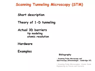
Scanning Tunneling Microscopy (STM). Short description Theory of 1-D tunneling Actual 3D barriers tip modeling atomic resolution Hardware Examples. Bibliography. Scanning Probe Microscopy and Spectroscopy (Wiesendanger, Cambridge UP)

E N D
Scanning Tunneling Microscopy (STM) Short description Theory of 1-D tunneling Actual 3D barriers tip modeling atomic resolution Hardware Examples Bibliography • Scanning Probe Microscopy and Spectroscopy (Wiesendanger, Cambridge UP) • Scanning Probe Microscopies: Atomic Scale Engineering by Forces and Currents
Scanning Tunneling Microscopy (STM) Piezolelectric Tube with Electrodes Tunneling Current Amplifier Distance Control and Scanning Unit Sample Tunneling Voltage Data Processing and Display Tip Sample Fundamental process: Electron tunneling
Electron tunneling Typical quantum phenomenon Tunneling definition Wave-particle impinging on barrier Probability of finding the particle beyond the barrier The particle have “tunneled” through it Role of tunneling in physics and knowledge development • Field emission from metals in high E field ( Fowler-Nordheim 1928) • Interband tunneling in solids (Zener 1934) • Field emission microscope (Müller 1937) • Tunneling in degenerate p-n junctions (Esaki 1958) • Perturbation theory of tunneling (Bardeen 1961) • Inelastic tunneling spectroscopy (Jaklevic, Lambe 1966) • Vacuum tunneling (Young 1971) • Scanning Tunneling Microscopy (Binnig and Rohrer 1982)
Electron tunneling Elastic Inelastic Energy conservation during the process Intial and final states have same energy Energy loss during the process Interaction with elementary excitations (phonons, plasmons) 3D 1D Planar Metal-Oxide-Metal junctions Scanning Tunneling Microscopy 3D Rectangular barriers Planar Metal-Oxide-Metal junctions Scanning Tunneling Microscopy Time independent Time-dependent Matching solutions of TI Schroedinger eq TD perturbation approach: (t) + first order pert. theory
Electron tunneling across 1-D potential barrier Time independent Region 1 Plane-wave of unit amplitude traveling to the right+ plane-wave of complex amplitude R traveling to the left Region 2 exponentially decaying wave plane-wave of complex amplitude T traveling to the right. Region 3 The solution in region 3 represents the “transmitted” wave
Electron tunneling across 1-D potential barrier Time independent Continuity conditions on and d/dz give At z=0 At z=s
Electron tunneling across 1-D potential barrier Time independent A square integrable (normalized) wave function has to remain normalized in time In a finite space region this conditions becomes Probability conservation Probability current
Electron tunneling across 1-D potential barrier Time independent Applying to our case Region 1 Region 3
Electron tunneling across 1-D potential barrier Time independent For strongly attenuating barriers xs >> 1 Large barrier height (i.e. small ) Exponential is leading contribution Barrier width s = 0.5 nm, V0 = 4 eV T ~ 10-5 Barrier width s = 0.4 nm, V0 = 4 eV T ~ 10-4 The transmission coefficient depends exponentially on barrier width Extreme sensitivity to z
Electron tunneling across 1-D potential barrier Time-dependent Ideal situation: incident state from left has some probability to appear on right … And we can calulate it… Real situation: At the surface the wavefunction is very complicated to calculate Different approach If barrier transmission is small, use perturbation theory But no easy way to write a perturbed Hamiltonian Approximate solutions of exact Hamiltonian within the barrier region l has to be matched with the correct solution of H for z 0 r has to be matched with the correct solution of H for z 0 Barrier width s = 0.5 nm, V0 = 4 eV xs ~ 10-5 Barrier width s = 0.4 nm, V0 = 4 eV xs ~ 10-4 Extreme sensitivity
Electron tunneling across 1-D potential barrier Time-dependent With the exact hamiltonian on left and right, we add a term HT representing the transition rate from l to r. HT = transfer Hamiltonian l,r = electron states at the left and right regions of the barrier HT is the term allowing to connect the right and left solutions Barrier width s = 0.5 nm, V0 = 4 eV xs ~ 10-5 Barrier width s = 0.4 nm, V0 = 4 eV xs ~ 10-4 Extreme sensitivity
Electron tunneling across 1-D potential barrier Time-dependent Choose the wavefunction Put into hamiltonian Barrier width s = 0.5 nm, V0 = 4 eV xs ~ 10-5 Barrier width s = 0.4 nm, V0 = 4 eV xs ~ 10-4 Extreme sensitivity
Electron tunneling across 1-D potential barrier Time-dependent The total probability over the space is Barrier width s = 0.5 nm, V0 = 4 eV xs ~ 10-5 Barrier width s = 0.4 nm, V0 = 4 eV xs ~ 10-4 Extreme sensitivity
Electron tunneling across 1-D potential barrier So the tunneling matrix element Mlr = Probability of tunneling from state l to state m Using the Fermi golden rule to obtain the transmitted current Density of states of the final state In general, the tunneling current contains information on the density of states of one of the electrodes, weighted by M But ………… each case has to calculated separately Barrier width s = 0.5 nm, V0 = 4 eV xs ~ 10-5 Barrier width s = 0.4 nm, V0 = 4 eV xs ~ 10-4 Extreme sensitivity
Electron tunneling across “real” 1-D potential barrier Time independent Introduce a more real potential: how to represent it? V(z) = slowly varying potential particle moving to the right with continuously varying wave-number (x) Try a solution
Electron tunneling across “real” 1-D potential barrier Time independent but This is true only if the first term is negligible, i.e. WKB approximation Wenzel Kramer Brillouin variation length-scale of x(z) (approximately the same as the variation length-scale of V(z)) must be much greater than the particle's de Broglie wavelength For E > V(z), x is real and the probability density is constant
Electron tunneling across “real” 1-D potential barrier Time independent Suppose the particle encounters a barrier between 0 < z1 < z2 so E < V(z) and x is imaginary Inside the barrier Neglect the exp growing part the probability density inside the barrier is the probability density at z1 is the probability density at z2 is
Electron tunneling across “real” 1-D potential barrier Time independent So the transmission coefficient becomes Tunneling probability very small The wavenumber is continuosly varying due to the potential: more real reasonable approximation for the tunneling probability if the incident << z (width of the potential barrier)
Electron tunneling across 1-D potential barrier Square barrier plane wave Exponential dependence of the transmission coefficient current depends on transfer matrix elements (containing exp. dependence) and on DOS Square barrier electron states Real barrier Plane waves True barrier representation if <<z Varying exponential dependence of the transmission coefficient Barrier width s = 0.5 nm, V0 = 4 eV xs ~ 10-5 Barrier width s = 0.4 nm, V0 = 4 eV xs ~ 10-4 Extreme sensitivity
Electron tunneling across 1-D metal electrodes insulator = vacuum The insulator defines the barrier Planar tunnel junctions Similar free electron like electrodes At equilibrium there is no net tunneling current and the Fermi level is aligned U=Bias voltage What is the net current if we apply a bias voltage? We must consider the Fermi distribution of electrons Barrier width s = 0.5 nm, V0 = 4 eV xs ~ 10-5 Barrier width s = 0.4 nm, V0 = 4 eV xs ~ 10-4 Extreme sensitivity
Electron tunneling across 1-D metal electrodes vz = electron speed along z n(vz)dvz = number of electrons/volume with vz T(Ez) = transmission coefficient of e- tunneling through V(z) e- with energy Ez =mvz2/2 f(E) = Fermi Dirac distribution n(vz)dvz = number of electrons/volume with vz Flux from electrode 1 to electrode 2 Barrier width s = 0.5 nm, V0 = 4 eV xs ~ 10-5 Barrier width s = 0.4 nm, V0 = 4 eV xs ~ 10-4 Extreme sensitivity
Electron tunneling across 1-D metal electrodes Flux from electrode 2 at positive potential U to electrode 1 Total number of electrons tunneling across junction tunneling current across junction The current depends on electron distribution Barrier width s = 0.5 nm, V0 = 4 eV xs ~ 10-5 Barrier width s = 0.4 nm, V0 = 4 eV xs ~ 10-4 Extreme sensitivity
Electron tunneling across 1-D metal electrodes since T is small when EF-Ez is large e- close to the Fermi level of the negatively biased electrode contribute more effectively to the tunneling current For positive U 2 is negligible so the net current flows from 1 to 2 For strongly attenuating barriers xs>>1 Exponential is leading contribution Barrier width s = 0.5 nm, V0 = 4 eV xs ~ 10-5 Barrier width s = 0.4 nm, V0 = 4 eV xs ~ 10-4 Extreme sensitivity
Electron tunneling across 1-D metal electrodes Applications of tunnel equation To perform the integration over the barrier define By integration it can be shown that At 0 K hence For strongly attenuating barriers xs>>1 Exponential is leading contribution Barrier width s = 0.5 nm, V0 = 4 eV xs ~ 10-5 Barrier width s = 0.4 nm, V0 = 4 eV xs ~ 10-4 Extreme sensitivity
Electron tunneling across 1-D metal electrodes integrating Current density flowing from electrode 1 to electrode 2 and vice versa If V = 0 dynamic equilibrium: current density flowing in either direction For positive U 2 is negligible so the net current flows from 1 to 2 For strongly attenuating barriers xs>>1 Exponential is leading contribution Barrier width s = 0.5 nm, V0 = 4 eV xs ~ 10-5 Barrier width s = 0.4 nm, V0 = 4 eV xs ~ 10-4 Extreme sensitivity
Electron tunneling across 1-D metal electrodes Low biases For strongly attenuating barriers xs>>1 Exponential is leading contribution Barrier width s = 0.5 nm, V0 = 4 eV xs ~ 10-5 Barrier width s = 0.4 nm, V0 = 4 eV xs ~ 10-4 Extreme sensitivity
Electron tunneling across 1-D metal electrodes Low biases Neglect second order contributions in U since At low biases the current varies linearly with applied voltage, i.e. Ohmic behavior Barrier width s = 0.5 nm, V0 = 4 eV xs ~ 10-5 Barrier width s = 0.4 nm, V0 = 4 eV xs ~ 10-4 Extreme sensitivity
Electron tunneling across 1-D metal electrodes High biases Electric field strength Put into general eq. evaluating a numerical factor (not included in eq) For this condition Second term of eq is negligible
Electron tunneling across 1-D metal electrodes High biases EF2 lies below the bottom of CB1 Hence e- cannot tunnel from 2 to 1 there are no levels available The situation is reversed for e- tunneling from 1 to 2: all available levels are empty analogous to field emission from a metal electrode: Fowler-Nordheim regime
Electron tunneling across 1-D potential barrier Square barrier, plane wave Exponential dependence of the transmission coefficient current depends on transfer matrix elements (containing exp. dependence) and on DOS Square barrier electron states Real barrier Plane waves Varying exponential dependence of the transmission coefficient Real barrier Metal electrodes Tunneling is most effective for e- close to Fermi level Low biases: Ohmic behavior Current flows from – to + electrode High biases: Fowler-Nordheim Barrier width s = 0.5 nm, V0 = 4 eV xs ~ 10-5 Barrier width s = 0.4 nm, V0 = 4 eV xs ~ 10-4 Extreme sensitivity
3-D potential barrier Square barrier electron states Real barrier Metal electrodes Join and extend the expression to have the equation for the tunneling current between a tip and a metal surface 1) Matrix element 0, Consider two many particle states of the sytem 0 = state with e- from state in left to state in right side of barrier 0, are eigenstates given by the WKB approximation Trick: both are good on one side only and inside the barrier but not on the other side of the barrier
3-D potential barrier is linear combination of one intial state 0 and numerous final states Put into Schroedinger equation and get a matrix with elements like Applyng a step function along z that is 1 only over barrier region the tunneling matrix element can be evaluated by integrating a current-like operator over a plane lying in the insulator slab The tunneling current depends on the electronic states of tip and surface Problem: calculation of the surface AND tip wavefunctions
3-D potential barrier Square barrier electron states Real barrier Metal electrodes Join the expression to have the equation for the tunneling current between a tip and a metal surface 2) Current density f(E) = Fermi function U = bias voltage applied to the sample M = tunneling matrix element = unperturbed electronic states of the surface = unperturbed electronic statesof the tip E (E) = energy of the state () in the absence of tunneling , are not eigenfunctions of the same H Not the many particle states
3-D potential barrier At low T one can consider only one directional tunneling
Low T + small (10 meV) applied bias voltage (U) For the Fermi function Low T + small (10 meV) applied bias voltage (U), E <EF
Tip modeling Low T + small applied bias voltage (U) Point like tip (unphysical) The matrix element is proportional to the probability density of surface states measured at r0 i.e. the local density of states at the Fermi level The image represents a contour map of the surface DOS at the Fermi level
Tip modeling Low T + small applied bias voltage (U) tip with radius R s-type only (quantum numbers l 0 neglected) wave functions with spherical symmetry to calculate the matrix element EF = Fermi energy r0 = center of curvature of the tip x = (2m)1/2/ ħ = decay rate = effective potential barrier height nt(EF) = density of states at the Fermi level for the tip Surface local density of states (LDOS) at EF measured at r0
Tip modeling The matrix element is integrated in a point of the barrier region s So the value of at r0 is no physically relevant, but it represents the lateral averaging due to finite tip size The exponential dependence comes from the matrix element STM is imaging the LDOS at the tip position Multiplied by the tip DOS
Tip modeling Sample wavefunctions have exponential decay in the z direction so little corrugation at s from surface Tip center position Surface local density of states (LDOS) at EF measured at r0 Au lattice parameter Calculated LDOS for Au(111) STM is imaging the LDOS at the tip position Multiplied by the tip DOS Low T + small applied bias voltage (U)
STM: atomic resolution We observe features with a spatial resolution better than 0.1 nm much lower of the tip curvature radius Smaller than spherical approximation of the tip wavefunctions (0.8 nm) Model failing to explain the most important feature of the STM: atomic resolution
STM: atomic resolution Why? Accuracy of perturbation theory: depends critically on the choice of the unperturbed wave functions, or the unperturbed Hamiltonians. For 3D tunneling the choice of unperturbed Hamiltonians is not unique. This is especially true for higher biases, in which the potential in the tunneling gap is not flat. Solution the unperturbed wave functions of sample and tip has to be different in the gap region • This unperturbed Hamiltonian minimizes the error introduced by neglecting the higher terms in the perturbation series. • The tip states are invariant as the bias changes, simplify calculations. • Easier estimation of bias distortion because the bias only affects the sample wave function, thus can be treated perturbatively
STM: atomic resolution To calculate I, the of the acting atom is expanded in terms of a complete set of eigenfunctions. Two choices: spherical coordinates parabolic coordinates Spherical coordinates are appropriate for describing atom loosely bonded on the tip Parabolic coordinates are appropriate for describing atom tightly bonded to the tip body. Calculated on the paraboloid
STM: atomic resolution Differences to Bardeen expression the wave functions are the eigenfunctions of tip and sample unperturbed Hamiltonians which are different in the gap region. It is valid only on the paraboloid that is the boundary of the tip body, not in the entire barrier region what is needed for calculating the tunneling matrix elements is the wave functions on the boundary of the tip
STM: atomic resolution On and outside boundary the tip satisfies the free electron Schroedinger equation decaying exponentially expand in term of the parabolic eigenfunctions with boundary conditions to be regular at r unperturbed wave functions of sample and tip different in the gap region The contribution of the tip wave function is determined only by its asymptotic values. The details of the tip wave functions near the center of the acting atom are not important On and inside boundary the sample satisfies the free electron Schroedinger equation decaying exponentially expand in term of the parabolic eigenfunctions with boundary conditions to be regular at center of the acting atom The contribution of the sample wave function is determined only by the values of the sample wave function in the vicinity of the center of the acting atom. The details of the sample wave functions outside the tip body are not important
STM: atomic resolution So M has to be integrated using orthonormal wavefunctions Spherical harmonics Bessel functions That leads to determine only the coefficients of the tip and sample expansion on orthonormal wavefunctions. The coefficients are determined by calculating the derivatives of the at the center of the acting atom M gives the correspondence between tip and sample wavefunctions
STM: atomic resolution For a choosen tip state, M changes and defines the relation to the coeffiecients of the surface Tip states s p d The tunneling matrix elements are related to the sample wavefunction derivatives
STM: atomic resolution The approximation on s state only is wrong the surface state of a real W tip extends into vacuum more than s and d states So the atomic resolution is given by the l 0 wave functions It is the most protruding electronic states that provides the J Not only the electron states at the Fermi level
STM: atomic resolution Reciprocity principle Is a basic microscopic symmetry ofSTM If the "acting" electronic state of the tip and the sample state are interchanged, the image should be the same. An image of microscopic scale may be interpreted either as by probing the sample state with a tip state or by probing the tip state with a sample state
Band structure effects z The electron energy in a solid depends on the band structure k is such that k+G=k The surface and tip define the direction z This may results in tunneling from surface or bulk states depending on their spatial extension Also T is changing as a function of E Electrons in states with large parallel wavevector tunnel less effectively